Propensity Score Matching: An Application on Observational Data

Wangila Collins; Wanjala Anjela; Muindi Jacinta

doi:doi:10.11648/j.ajmcm.20240903.12

Research Article |

| Peer-Reviewed

Propensity Score Matching: An Application on Observational Data

Wangila Collins

, Wanjala Anjela^*

, Muindi Jacinta

Published in American Journal of Mathematical and Computer Modelling (Volume 9, Issue 3)

Received: 26 October 2024 Accepted: 12 November 2024 Published: 3 December 2024

Views: Downloads:

Download PDF

Share This Article

Twitter
Linked In
Facebook

Abstract

The study aimed to determine the survival rate of first-class passengers using the Titanic dataset from Kaggle. Descriptive statistics revealed that first class passengers had way more chance to survive as compared to other classes, which underscores the role of socioeconomic status in determining chances of survival. Evaluation metrics, which assess model performance independently for male and female cohorts, shed light on gender specific projected accuracy. The analysis of propensity scores matching data for male and female passengers separately ensured that each gender category had control groups and treatments that were equally distributed. It was discovered that women had higher survival rates compared to men and these findings also identified disparities in the levels of surviving among genders. Improvements in covariate balance were indicated by post-matching statistics for both the male and female cohorts, indicating that the matching process was successful for both genders. The treatment effect estimates for male and female passengers were computed independently, and the findings showed that a number of characteristics significantly improved the survival rates for each gender group. The overall results of the study emphasized how important it is to include gender when analyzing survival outcomes using the Titanic dataset. In addition, age was suggested as an important factor whereby young people had higher chances of being saved.

Published in	American Journal of Mathematical and Computer Modelling (Volume 9, Issue 3)
DOI	10.11648/j.ajmcm.20240903.12
Page(s)	68-77
Creative Commons	This is an Open Access article, distributed under the terms of the Creative Commons Attribution 4.0 International License (http://creativecommons.org/licenses/by/4.0/), which permits unrestricted use, distribution and reproduction in any medium or format, provided the original work is properly cited.
Copyright	Copyright © The Author(s), 2024. Published by Science Publishing Group

Keywords

Propensity Score Matching, Survival Rates, Observational Data, Treatment and Control Groups

1. Introduction

In the realm of evaluation problems, datasets often arise from non-randomized observational studies rather than randomized trials, introducing challenges in estimating treatment effects due to the absence of random assignment. Propensity score matching (PSM), a technique to reduce bias in observational datasets, was first presented by Rosenbaum and Rubin (1983).

Propensity score matching operates on the principle of creating balance between treated and untreated groups by matching individuals based on their estimated propensity scores

[1]

. The propensity score, representing the probability of receiving treatment given observed covariates, serves as a crucial intermediary. The purpose of PSM is to improve the validity of treatment effect estimations by simulating a randomized trial by minimizing the observed characteristic imbalance.

This methodology is becoming more and more popular in two key areas: the assessment of economic policy measures and medical trials. Within the medical domain, where conducting randomized trials may pose practical or ethical difficulties, PSM provides a way to manage the intricacies of observational data and provide more reliable treatment effect estimates

[2]

. PSM also offers policymakers a useful tool for evaluating how different policies affect different outcomes, which helps them make well-informed decisions. This is especially true in the area of economic policy.

Rosenbaum and Donald B. Rubin

[3]

refer to observational studies as research methods where investigators observe subjects in their natural environment without intervening or manipulating any variables. These studies aim to assess asociations between variables or investigate causal relationships without the use of experimental control. Observational studies are essential in epidemiology, social sciences, and other fields where conducting randomized controlled trials may be impractical or unethical.

Propensity score matching consequently still has two key goals. Creating matched groups with identical observable features is the first step towards reducing bias and successfully controlling for any confounding variables (Rosenbaum & Rubin, 1983, 1984)

[4]

. In order to enable researchers to derive more trustworthy conclusions from non-randomized datasets, it also aims to strengthen the validity of treatment effect estimates in observational studies. Propensity score matching is a flexible methodology that may be applied to a wide range of study topics. It is still essential for enhancing causal inference and raising the level of methodological rigor in assessments.

2. Methodology

There are six steps involved in doing propensity score matching. The selection of variables, propensity score models, matching distances and algorithms, treatment effect estimation, and match quality diagnosis are just a few of the decisions that need to be made at each stage see, for example

[1, 5-7]

2.1. Select Variables

The first step in the propensity score matching procedure is selecting the variables (sometimes referred to as "covariates") to be included in the model. A collection of factors connected to an intervention’s self-selection by participants is the best source of propensity scores. The variables serve as predictors of intervention participation when propensity scores are produced by logistic regression (0/1). Based on the propensity score which is established by the multivariate distribution of the variables—the researcher may balance the intervention and comparison group (Stuart & Rubin, 2008a). The precision of conclusions a researcher may draw on the outcomes of an intervention is influenced by the inclusion or absence of important variables

[8, 9]

. It is important to consider characteristics that are conceptually associated with self-selection when selecting covariates

[8, 9]

2.2. Propensity Score Estimation

A multivariate composite of the variables can be produced by calculating propensity scores using a variety of methods (For instance, discriminant analysis, Mahalanobis distance, logistic regression, etc.). There are several ways to go about it, depending on how many degrees are offered (for example, providing two program variations with different criteria for student investment vs providing one honors program). Logistic regression is the most widely used method for producing propensity scores

[10]

The propensity score, denoted as e(X), is the conditional probability of receiving treatment (T = 1) given the observed covariates (X):

e(X) =P(T= 1|X)(1)

Commonly, this is estimated using logistic regression:

logit(e(X)) =β₀+β₁X₁+β₂X₂+...+β_kX_k(2)

Regardless of the approach used, all individuals must have a nonzero likelihood of taking part in the intervention for propensity score matching to be applied

[11]

2.3. Propensity Score Matching

Matching based on propensity scores involves assembling groups of individuals who have and have not received treatment, with similar matching scores

[3, 4]

This method simplifies the estimation of the Average Treatment Effect for the Treated (ATT)

[12]

. To guarantee that the propensity score values of treated and untreated participants are equal, one-to-one or pair matching is the most common approach used in propensity score matching. Alternative techniques exist even though one-to-one matching is a commonly employed strategy. After a matched sample has been established, a direct comparison of the outcomes of treated and untreated participants within the matched sample is necessary to estimate the treatment effect. The treatment impact for continuous outcomes, such as a depression scale, is found by dividing the mean result for treated patients in the matched sample by the mean outcome for untreated subjects

[3]

. When an outcome, such the presence or absence of self-reported depression, is dichotomous, the treatment effect is ascertained by contrasting the percentages of persons in the treated and untreated groups who experience the event in the relevant sample.

2.4. Balance Checking

The methods presented here are intended to be used in the context of propensity score-based one-to-one matching. You can find adjustments for propensity score use in many-to-one matching elsewhere

[11]

. These methods can be readily adjusted for use in Inverse Probability of Treatment Weighting (IPTW) utilizing the propensity score and stratification based on the propensity score

[13, 14]

. Further information may be found in other sources about diagnostics evaluating goodness-of-fit for covariate modification with the propensity score

[15]

2.5. Balance Comparison

2.5.1. Numerical Balance Analysis

The means or medians of continuous variables and the distribution of their categorical equivalents across the two groups should be compared in order to evaluate the comparability of treated and untreated participants in the matched sample. An effective metric for comparing the means of continuous and binary variables between treatment groups is the standardized difference

[16]

. Multilevel categorical variables can be represented using a set of binary indicator variables

[17]

Standardized Mean Differences (SMD) can be employed both before and after matching to evaluate the covariate balance:

SMD = \frac{\bar{X} treated - \bar{X} control}{q \frac{\frac{s^{2} + s^{2}}{treated control}}{2}}

(3)

Where: X¯treated and X¯control are the means of the covariate for the treated and control groups, respectively.

S_{treated}^{2} and S_{control}^{2}

are the variances of the covariate for the treated and control groups, respectively.

A standardized measure of the mean difference between the two groups represented as standard deviations is provided by the SMD. A small SMD (around zero) denotes a fair degree of group balance and suggests similarity in the covariate distributions.

To consider the factors balanced, researchers usually strive for SMD values below a specific threshold (e.g., 0.1 or 0.2). Adjustments or other matching strategies could be required if the SMD is large before matching, indicating an imbalance in the variables. Comparing the SMD values after matching aids in determining whether or not the matching procedure was successful in establishing balance.

2.5.2. Balance Diagnosis Visually

Using density plots made using the ggplot2 package is a simple method of visually comparing distributions

[18]

. R gives an example where the distribution of variables (Y1-Y6) is compared for two university student groups: those who took part in the honors program (referred to as the "treatment") and those who did not ("control"). Keep in mind that the covariates’ distribution differs by group and between variables.

2.6. Outcome Analysis

To adhere to propensity score matching best practices,

[1]

pointed out that adding outcome variables after all matches have been made is essential.

The treatment effect (τ) may be calculated by a comparison of the mean results of the treatment (Y₁) and control (Y₀) groups:

T=Y¯₁− Y¯₀(4)

The effect of the intervention may be calculated once a comparison group has been established via the use of propensity score matching procedures. Estimates of the treatment effects can be made, depending on the study question, for either:

The intervention’s effect on the participants alone (average treatment effect on the treated)

To conclude the program’s possible effects on the student body as a whole (average treatment effect;

[5-7]

. The average treatment impact on the treated (ATT) may be readily computed if the objective is to evaluate treatment effects for only the participants in the intervention. The treatment group for whom the researcher has data in the context of ATT represents the whole population.

Average Treatment Effect on the Treated (ATT)

It is simple to estimate the average treatment effect on the treated (ATET) if the objective is to evaluate treatment effects on those who receive the treatment. The total population of interest in the context of ATT is represented by the treatment group for whom the researcher has data (Austin, 2011

[11]

; Imbens, 2004)

[12]

ATT =E[Y_i¹− Y_i⁰|T_i= 1],where(5)

T_i is the treatment indicator.

Average Treatment Effect on the Control (ATC)

The average effect of the treatment on those who do not receive the treatment (control group).

ATC =E[Y_i¹− Y_i⁰|T_i= 0],where(6)

T_i is the treatment indicator.

Average Treatment Effect (ATE):

Alternatively, conclusions about an intervention’s impacts that would apply to all students, regardless of whether they got therapy, might be the main objective. i.e., The average effect of the treatment on the entire population. The average treatment effect (ATE) in this case is calculated as the average effects weighted by the baseline characteristics of the general population as determined by the covariates (Ho et al., 2007)

[7]

. Two techniques for determining ATE by weighting the propensity scores are stratification and inverse probability of treatment weighting (Austin, 2011)

[11]

ATE =E[Y_i¹− Y_i⁰](7)

where

Y_i ¹ is the potential outcome if treated,

Y_i ⁰ is the potential outcome if not treated,

and the expectation is taken over the entire population.

3. Data Analysis

3.1. Descriptive Statistics

We will utilize the widely available Titanic dataset from Kaggle in our investigation. The goal is to determine the first-class cabin survival rate.

Table 1. Descriptive Statistics for is pclass1.

Max	Count	Mean	Std	Min	25%	50%	75%
False	528.00	0.32	0.47	0.00	0.00	0.00	0.00
1.00
True	186.00	0.66	0.48	0.00	0.00	1.00	1.00
1.00

The survival rate of first-class passengers (the treatment group) is 66%, whereas that of other class passengers (the control group) is 32%.

Download: Download full-size image

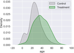
Figure 1. Treatment group comparison based on age.

In figure 1 the control group has younger passengers in comparison to the treatment.

Download: Download full-size image

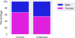
Figure 2. Gender distribution in the Titanic dataset.

There are also more females in the treatment group in figure 2. It would be naive to assume that the treatment is the reason for the difference in survival rate at this point, as the confounding factors are not equal across the two groups.

3.2. Propensity Model

Table 2. Propensity model for Titanic data.

Survived	is_pclass1	is male	Age	Proba	Logit	Pred
0	0	False	True	22.00	0.12	-1.98
0
1	1	True	False	38.00	0.44	-0.22
0
1	0	False	False	26.00	0.28	-0.96
0
1	1	True	False	35.00	0.40	-0.41
0
0	0	False	True	35.00	0.24	-1.18
0

In Table 2 the propensity model predicts the likelihood of receiving the treatment given the confounders.

Since we aren’t creating a predictive model, I didn’t split the data into a train and test split. The propensity score indicates the likelihood that a patient will receive the treatment in light of the confounders. I included the logit transformation.

3.2.1. Metrics for Model Evaluation

Table 3. Metrics for Model Evaluation.

Metric	Value
Accuracy	0.7591
ROC	AUC 0.7467
F1-score	0.3435

Table 3 presents the evaluation metrics for the classification model, providing a comprehensive overview of its performance. The accuracy metric, which measures the proportion of correctly classified instances, indicates that the model produced results with an accuracy of 0.7591, implying that approximately 75.91% of the cases had accurate classifications. This suggests a reasonably reliable performance of the model in distinguishing between the classes.

Additionally, 0.7467 is given for the ROC AUC score, which is a key indicator of the model’s capacity to distinguish between positive and negative classifications. A higher score denotes greater discrimination, and this one indicates that the model does a respectable job of differentiating between the classes. Calculated to be 0.3435, the F1-score is another important statistic that strikes a compromise between recall and accuracy. The score indicates possible areas for the model’s performance to be improved by highlighting the balance between recall (the model’s ability to capture all relevant instances) and accuracy (the model’s ability to identify relevant examples).

3.2.2. Confusion Matrix

Table 4. Results of Confusion Matrix.

	False	True
False	497	31
True	141	45

Table 4 shows the model distribution of its accurate and wrong predictions. From confusion matrix we can clearly see that there were 497 true negatives, 45 true positives, 31 false positives, and 141 false negatives out of the total cases. This dissection offers a thorough comprehension of the model’s performance for various predicted outcomes. The model can accurately classify instances and distinguish between classes, as evidenced by its ROC AUC and reasonable accuracy. However, its comparatively lower F1-score implies that there is room for development in the model’s ability to balance precision and recall.

Download: Download full-size image

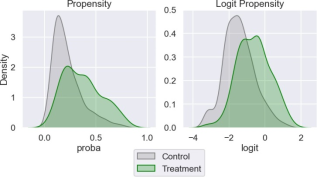
Figure 3. Propensity score and logit propensity.

The propensity score makes it much easier to locate comparable records than the several dimensions (confounders). This may bring to mind methods for reducing dimensionality. It is counterbalanced by a propensity score. This implies that the confounders’ distribution between matched records will probably be comparable if records are matched using the propensity score.

3.3. Propensity Score Matching

3.3.1. Matching Entries in the Titanic Dataset Based on Their Propensity Scores

Table 5. Matching records in the Titanic data set with propensity score.

Distance	Survived	is_Pclass1	is Male	Age	Proba	Logit	Pred	Match
243	1	True	True	0.92	0.04	-3.27	0	59.00
-0.01
357	1	True	True	4.00	0.04	-3.08	0	154.00
-0.06
639	1	True	True	11.00	0.07	-2.65	0	44.00
0.00
240	0	True	False	2.00	0.08	-2.44	0	94.00
0.00
437	1	True	True	17.00	0.09	-2.28	0	346.00
0.00
74	0	True	True	71.00	0.74	1.04	1	91.00
-0.03
293	1	True	False	60.00	0.76	1.13	1	91.00
-0.12
662	1	True	False	62.00	0.78	1.26	1	91.00
-0.25
221	1	True	False	63.00	0.79	1.32	1	679.00
-0.09
498	1	True	True	80.00	0.83	1.60	1	679.00
-0.37

Table 5 presents matched records from the Titanic dataset, organized by propensity scores. Each entry corresponds to a passenger, indicating survival status, class, gender, age, propensity score, and matching specifics like predicted treatment assignment, match index, and propensity score distance. These details facilitate the evaluation of propensity score matching’s efficacy in establishing balanced treatment and control cohorts for causal analysis.

3.3.2. Matched Data

Table 6. Matched Data.

Distance	Survived	is_Pclass1	is_Male	Age	Proba	Logit	Pred	Match
0	0	1	True	True	0.92	0.04	-3.27	0
59.00	-0.01
1	1	1	True	True	4.00	0.04	-3.08	0
154.00	-0.06
2	2	1	True	True	11.00	0.07	-2.65	0
44.00	0.00
3	3	0	True	False	2.00	0.08	-2.44	0
94.00	0.00
4	4	1	True	True	17.00	0.09	-2.28	0
346.00	0.00
367	367	0	False	True	70.50	0.73	1.01	1
NaN	NaN
368	368	0	False	True	70.50	0.73	1.01	1
NaN	NaN
369	369	0	False	True	70.50	0.73	1.01	1
NaN	NaN
370	370	0	False	True	74.00	0.77	1.23	1
NaN	NaN
371	371	0	False	True	74.00	0.77	1.23	1
NaN	NaN

Table 6 shows that the confounding factors indicate that this new control group is similar to the treatment group.

3.3.3. Evaluating the Quality of Matching

Table 7. Evaluating the quality of matching.

	age_t	is_male_t	survived_t	match	age_c	is_male_c	survived_c
243	0.92	True	1	59.00	0.83	True	1
357	4.00	True	1	154.00	3.00	True	1
639	11.00	True	1	44.00	11.00	True	0
240	2.00	False	0	94.00	2.00	False	0
437	17.00	True	1	346.00	17.00	True	0
74	71.00	True	0	91.00	70.50	True	0
293	60.00	False	1	91.00	70.50	True	0
662	62.00	False	1	91.00	70.50	True	0
221	63.00	False	1	679.00	74.00	True	0
498	80.00	True	1	679.00	74.00	True	0

Notably, treatment records 293, 662, and 221 show little resemblance to their control matches among these ten samples. For the other seven cases, though, the matches appear very similar.

3.3.4. Logit and Age Before and After Matching

Table 8. Logit and Age Before and After Matching.

Logit \| After matching
	count	mean	std	min	25%	50%	75%	max
is_pclass1 False	528.00	-1.43	0.85	-3.31	-2.04	-1.48	-0.90	1.32
is_pclass1 True	186.00	-0.63	0.91	-3.27	-1.26	-0.58	-0.01	1.60
Logit \| After matching
	count	mean	std	min	25%	50%	75%	max
is_pclass1 False	186.00	-0.65	0.88	-3.28	-1.26	-0.61	-0.04	1.23
is_pclass1 True	186.00	-0.63	0.91	-3.27	-1.26	-0.58	-0.01	1.60
Age \| Before matching
	count	mean	std	min	25%	50%	75%	max
is_pclass1 False	528.00	26.69	13.18	0.42	19.00	26.00	34.00	74.00
is_pclass1 True	186.00	38.23	0.92	14.80	27.00	37.00	49.00	80.00
Age \| After matching
	count	mean	std	min	25%	50%	75%	max
is_pclass1 False	186.00	37.84	15.50	0.83	27.00	36.00	49.75	74.00
is_pclass1 True	186.00	38.23	14.80	0.92	27.00	37.00	49.00	80.00

For the logit variable, before matching, the mean logit values for the groups not in the first class (is_pclass1 False) and in the first class (is_pclass1 True) are -1.43 and -0.63, respectively. After matching, the mean logit values shift slightly to -0.65 and -0.63 for the respective groups. While there is a slight change in the means, the standard deviations and quartile values also show modest alterations. Overall, the changes indicate a degree of improvement in achieving balance between the treatment and control groups after the matching process for the logit variable.

Considering the age variable, the groups not in the first class and those in the first class had mean age values of 26.69 and 38.23, respectively, before matching. After matching, the relevant groups’ mean ages are 38.23 and 37.84, respectively. The averages, standard deviations, and quartile values all show minor changes, much like the logit variable does, indicating a respectable im- provement in covariate balance following matching.

In conclusion, after applying propensity score matching, the data show a tendency toward greater similarity for both the age and logit variables between the treatment and control groups. These modifications strengthen the validity of later causal inferences about the influence of being in the first class on the given outcomes by enhancing the comparability and making it more balanced.

Download: Download full-size image

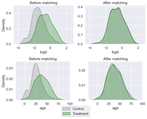
Figure 4. Control and treatment distributions before and after matching.

3.3.5. Proportions Before and After Matching

Table 9. Proportions Before Matching.

	is_male False	is_male True
is_pclass1 False	0.33	0.67
is_pclass1 True	0.46	0.54

Table 10. Proportions After Matching.

	is_male False	is_male True
is_pclass1 False	0.46	0.54
is_pclass1 True	0.46	0.54

The percentage of male and female passengers in each class is shown in Table 9 before matching. The proportion of males and females in the control group (is_pclass1 False) is 0.33 and 0.67, respectively. In comparison, the proportion of males and females in the treatment group (is_pclass1 True) is 0.46 and 0.54, respectively. The male and female proportions in each class equalize after matching, as indicated by Table 10, with a male percentage of 0.46 and a female proportion of 0.54. This balance shows that the treatment and control groups’ gender distributions were successfully matched.

Download: Download full-size image

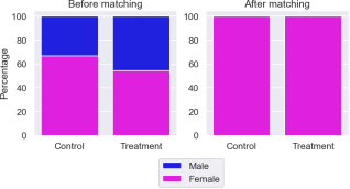
Figure 5. Bar graphs the distribution of gender before and after matching.

3.4. Balance Comparison

Table 11. Standardized Mean Differences (SMD) for Covariates.

Variable	SMD Value
Age	0.0258
is_male	0.0000

The standardized difference in means for each covariate between the treatment and control groups is measured by the SMD values. In propensity score matching, lower SMD values often suggest greater group balance and similarity concerning the relevant covariate. The age variable’s SMD (0.0258) indicates a tiny, standardized difference, suggesting that the age variable has been fairly balanced during the matching process. Furthermore, the fact that is_male’s SMD is nearly zero (0.0000) suggests that the matching process has successfully balanced the gender distribution of is_male between the treatment and control groups. These findings collectively imply that the matching procedure was successful in obtaining equilibrium among these factors.

3.5. Outcome Analysis

3.5.1. Descriptive Statistics on the Outcome

Table 12. Descriptive statistics on the outcome.

is_pclass1	Mean	Standard Deviation	Count
False	0.36	0.48	186
True	0.66	0.48	186

The Average Treatment Effect on Treated (ATT): 0.2957.

ATT suggests that, on average, individuals who received a first-class passenger cabin experienced a 29.57% increase in their chance of survival compared to those who did not receive the first-class cabin, after accounting for all confounding factors.

3.5.2. Treatment Effect Estimates: Matching

Table 13. Treatment Effect Estimates: Matching.

	Est.	S.e.	z	[95% Conf. int.]
ATE	0.284	0.056	5.042	(0.173, 0.394)
ATC	0.277	0.064	4.313	(0.151, 0.403)
ATT	0.302	0.057	5.258	(0.189, 0.414)

The average treatment effect (ATE) of 0.284 suggests that, after accounting for confounding variables, travelers who had a first-class cabin had an overall better probability of surviving than those who did not.

This had an overall positive impact on survival across all passengers. For the control group (ATC), the estimated treatment effect of 0.277 implies that passengers without a first-class cabin experienced a positive impact on their survival status. This suggests that factors other than the first-class cabin also contributed to an increased chance of survival among this group. On the other hand, the Average Treatment Effect on the Treated (ATT) of 0.302 suggests a positive impact on survival among passengers who had a first-class cabin. This indicates that having a first-class cabin was associated with a higher chance of survival. It may be concluded that, on average, the first-class cabin had a substantial impact on the survival rates of Titanic passengers since all treatment effects had statistically significant p-values that lend credence to these estimates.

4. Conclusion and Recommendations

The research revealed that first class passengers had way more chance to survive as compared to other classes, which underscores the role of socioeconomic status in determining chances of survival. According to a study on gender, women had higher survival rates compared to men and these findings also identified disparities in the levels of surviving among genders. Also, age has been suggested as an important factor whereby young people had higher chances of being saved. Propensity score matching can be complemented with using other matching techniques such as Mahalanobis distance or propensity score weighting for a more insightful sensitivity analysis on studying the robustness of results.

In addition, further investigation regarding treatment heterogeneity may also involve subgroup analyzes based on age cohorts or gender categories that emphasize treatment effects within specific demographic groups. Additionally, the robustness of causal claims made through observational data could be affirmed by conducting sensitivity tests like Rosenbaum bounds or sensitivity analyses such as E-values to examine the influence of non-observed confounders. By integrating multiple approaches in sensitivity analysis, the validity for causal interpretations can be strengthened by giving a comprehensive assessment on how stable and reliable are the findings derived from this study.

Abbreviations

ATE	Average Treatment Effect
SMD	Standardized Mean Differences
ATT	Average Treatment Impact on the Treated
ATC	Average Treatment Effect on the Control

Author Contributions

Wangila Collins: Conceptualization, Funding acquisition, Methodology, Resources

Wanjala Anjela: Formal Analysis, Funding acquisition, Methodology, Visualization, Writing – review & editing

Muindi Jacinta: Data curation, Funding acquisition, Methodology, Visualization, Writing – original draft

Conflicts of Interest

The authors declare no conflicts of interest.

References

[1]	H. Harris and S. J. Horst, “A brief guide to decisions at each step of the propensity score matching process,” Practical Assessment, Research, and Evaluation, vol. 21, no. 1, p. 4, 2019.
[2]	A. S. Jones, R. B. D’Agostino Jr, E. W. Gondolf, and A. Heckert, “Assessing the effect of batterer program completion on reassault using propensity scores,” Journal of Interpersonal Violence, vol. 19, no. 9, pp. 1002–1020, 2004.
[3]	P. R. Rosenbaum and D. B. Rubin, “The central role of the propensity score in observational studies for causal effects,” Biometrika, vol. 70, no. 1, pp. 41–55, 1983.
[4]	P. R. Rosenbaum and D. B. Rubin, “The bias due to incomplete matching,” Biometrics, pp. 103–116, 1985.
[5]	M. Caliendo and S. Kopeinig, “Some practical guidance for the implementation of propensity score matching,” Journal of economic surveys, vol. 22, no. 1, pp. 31–72, 2008.
[6]	X. S. Gu and P. R. Rosenbaum, “Comparison of multivariate matching methods: Structures, distances, and algorithms,” Journal of Computational and Graphical Statistics, vol. 2, no. 4, pp. 405–420, 1993.
[7]	D. E. Ho, K. Imai, G. King, and E. A. Stuart, “Matching as nonparametric preprocessing for reducing model dependence in parametric causal inference,” Political analysis, vol. 15, no. 3, pp. 199–236, 2007.
[8]	M. A. Brookhart, S. Schneeweiss, K. J. Rothman, R. J. Glynn, J. Avorn, and T. Stürmer, “Variable selection for propensity score models,” American journal of epidemiology, vol. 163, no. 12, pp. 1149–1156, 2006.
[9]	A. W. Steiner, J. M. Lattimer, and E. F. Brown, “The equation of state from observed masses and radii of neutron stars,” The Astrophysical Journal, vol. 722, no. 1, p. 33, 2010.
[10]	E. A. Stuart, “Matching methods for causal inference: A review and a look forward,” Statistical science: a review journal of the Institute of Mathematical Statistics, vol. 25, no. 1, p. 1, 2010.
[11]	P. C. Austin, “An introduction to propensity score methods for reducing the effects of confounding in observational studies,” Multivariate behavioral research, vol. 46, no. 3, pp. 399–424, 2011.
[12]	G. W. Imbens, “Nonparametric estimation of average treatment effects under exogeneity: A review,” Review of Economics and statistics, vol. 86, no. 1, pp. 4–29, 2004.
[13]	H. J. Schmoll, R. Souchon, S. Krege, P. Albers, J. Beyer, C. Kollmannsberger, S. Fossa, N. Skakkebaek, R. De Wit, K. Fizazi, et al., “European consensus on diagnosis and treatment of germ cell cancer: a report of the european germ cell cancer consensus group (egcccg),” Annals of Oncology, vol. 15, no. 9, pp. 1377–1399, 2004.
[14]	S. L. Morgan and J. J. Todd, “A diagnostic routine for the detection of consequential heterogeneity of causal effects,” Sociological Methodology, vol. 38, no. 1, pp. 231–281, 2008.
[15]	T. Young, L. Finn, P. E. Peppard, M. Szklo-Coxe, D. Austin, F. J. Nieto, R. Stubbs, and K. M. Hla, “Sleep disordered breathing and mortality: eighteen-year follow-up of the wisconsin sleep cohort,” Sleep, vol. 31, no. 8, pp. 1071–1078, 2008.
[16]	B. K. Flury and H. Riedwyl, “Standard distance in univariate and multivariate analysis,” The American Statistician, vol. 40, no. 3, pp. 249–251, 1986.
[17]	P. C. Austin, “Balance diagnostics for comparing the distribution of baseline covariates between treatment groups in propensity-score matched samples,” Statistics in medicine, vol. 28, no. 25, pp. 3083–3107, 2009.
[18]	A. Buja, D. Cook, H. Hofmann, M. Lawrence, E.-K. Lee, D. F. Swayne, and H. Wickham, “Statistical inference for exploratory data analysis and model diagnostics,” Philosophical Transactions of the Royal Society A: Mathematical, Physical and Engineering Sciences, vol. 367, no. 1906, pp. 4361–4383, 2009.

Cite This Article

Plain Text BibTeX RIS

APA Style

Collins, W., Anjela, W., Jacinta, M. (2024). Propensity Score Matching: An Application on Observational Data. American Journal of Mathematical and Computer Modelling, 9(3), 68-77. https://doi.org/10.11648/j.ajmcm.20240903.12

Copy | Download

ACS Style

Collins, W.; Anjela, W.; Jacinta, M. Propensity Score Matching: An Application on Observational Data. Am. J. Math. Comput. Model. 2024, 9(3), 68-77. doi: 10.11648/j.ajmcm.20240903.12

Copy | Download

AMA Style

Collins W, Anjela W, Jacinta M. Propensity Score Matching: An Application on Observational Data. Am J Math Comput Model. 2024;9(3):68-77. doi: 10.11648/j.ajmcm.20240903.12

Copy | Download

@article{10.11648/j.ajmcm.20240903.12,
  author = {Wangila Collins and Wanjala Anjela and Muindi Jacinta},
  title = {Propensity Score Matching: An Application on Observational Data
},
  journal = {American Journal of Mathematical and Computer Modelling},
  volume = {9},
  number = {3},
  pages = {68-77},
  doi = {10.11648/j.ajmcm.20240903.12},
  url = {https://doi.org/10.11648/j.ajmcm.20240903.12},
  eprint = {https://article.sciencepublishinggroup.com/pdf/10.11648.j.ajmcm.20240903.12},
  abstract = {The study aimed to determine the survival rate of first-class passengers using the Titanic dataset from Kaggle. Descriptive statistics revealed that first class passengers had way more chance to survive as compared to other classes, which underscores the role of socioeconomic status in determining chances of survival. Evaluation metrics, which assess model performance independently for male and female cohorts, shed light on gender specific projected accuracy. The analysis of propensity scores matching data for male and female passengers separately ensured that each gender category had control groups and treatments that were equally distributed. It was discovered that women had higher survival rates compared to men and these findings also identified disparities in the levels of surviving among genders. Improvements in covariate balance were indicated by post-matching statistics for both the male and female cohorts, indicating that the matching process was successful for both genders. The treatment effect estimates for male and female passengers were computed independently, and the findings showed that a number of characteristics significantly improved the survival rates for each gender group. The overall results of the study emphasized how important it is to include gender when analyzing survival outcomes using the Titanic dataset. In addition, age was suggested as an important factor whereby young people had higher chances of being saved.
},
 year = {2024}
}

Copy | Download

TY  - JOUR
T1  - Propensity Score Matching: An Application on Observational Data

AU  - Wangila Collins
AU  - Wanjala Anjela
AU  - Muindi Jacinta
Y1  - 2024/12/03
PY  - 2024
N1  - https://doi.org/10.11648/j.ajmcm.20240903.12
DO  - 10.11648/j.ajmcm.20240903.12
T2  - American Journal of Mathematical and Computer Modelling
JF  - American Journal of Mathematical and Computer Modelling
JO  - American Journal of Mathematical and Computer Modelling
SP  - 68
EP  - 77
PB  - Science Publishing Group
SN  - 2578-8280
UR  - https://doi.org/10.11648/j.ajmcm.20240903.12
AB  - The study aimed to determine the survival rate of first-class passengers using the Titanic dataset from Kaggle. Descriptive statistics revealed that first class passengers had way more chance to survive as compared to other classes, which underscores the role of socioeconomic status in determining chances of survival. Evaluation metrics, which assess model performance independently for male and female cohorts, shed light on gender specific projected accuracy. The analysis of propensity scores matching data for male and female passengers separately ensured that each gender category had control groups and treatments that were equally distributed. It was discovered that women had higher survival rates compared to men and these findings also identified disparities in the levels of surviving among genders. Improvements in covariate balance were indicated by post-matching statistics for both the male and female cohorts, indicating that the matching process was successful for both genders. The treatment effect estimates for male and female passengers were computed independently, and the findings showed that a number of characteristics significantly improved the survival rates for each gender group. The overall results of the study emphasized how important it is to include gender when analyzing survival outcomes using the Titanic dataset. In addition, age was suggested as an important factor whereby young people had higher chances of being saved.

VL  - 9
IS  - 3
ER  -

Copy | Download

Author Information

Wangila Collins

Department of Mathematics, University of Nairobi, Nairobi, Kenya

Contact Email

http://orcid.org/0009-0004-5073-7622
Wanjala Anjela

Department of Mathematics, University of Nairobi, Nairobi, Kenya

Contact Email

http://orcid.org/0009-0001-7063-9526
Muindi Jacinta

Department of Mathematics, University of Nairobi, Nairobi, Kenya

Contact Email

http://orcid.org/0009-0002-2469-0141

Download PDF

Plain Text BibTeX RIS

APA Style

Collins, W., Anjela, W., Jacinta, M. (2024). Propensity Score Matching: An Application on Observational Data. American Journal of Mathematical and Computer Modelling, 9(3), 68-77. https://doi.org/10.11648/j.ajmcm.20240903.12

Copy | Download

ACS Style

Collins, W.; Anjela, W.; Jacinta, M. Propensity Score Matching: An Application on Observational Data. Am. J. Math. Comput. Model. 2024, 9(3), 68-77. doi: 10.11648/j.ajmcm.20240903.12

Copy | Download

AMA Style

Collins W, Anjela W, Jacinta M. Propensity Score Matching: An Application on Observational Data. Am J Math Comput Model. 2024;9(3):68-77. doi: 10.11648/j.ajmcm.20240903.12

Copy | Download

@article{10.11648/j.ajmcm.20240903.12,
  author = {Wangila Collins and Wanjala Anjela and Muindi Jacinta},
  title = {Propensity Score Matching: An Application on Observational Data
},
  journal = {American Journal of Mathematical and Computer Modelling},
  volume = {9},
  number = {3},
  pages = {68-77},
  doi = {10.11648/j.ajmcm.20240903.12},
  url = {https://doi.org/10.11648/j.ajmcm.20240903.12},
  eprint = {https://article.sciencepublishinggroup.com/pdf/10.11648.j.ajmcm.20240903.12},
  abstract = {The study aimed to determine the survival rate of first-class passengers using the Titanic dataset from Kaggle. Descriptive statistics revealed that first class passengers had way more chance to survive as compared to other classes, which underscores the role of socioeconomic status in determining chances of survival. Evaluation metrics, which assess model performance independently for male and female cohorts, shed light on gender specific projected accuracy. The analysis of propensity scores matching data for male and female passengers separately ensured that each gender category had control groups and treatments that were equally distributed. It was discovered that women had higher survival rates compared to men and these findings also identified disparities in the levels of surviving among genders. Improvements in covariate balance were indicated by post-matching statistics for both the male and female cohorts, indicating that the matching process was successful for both genders. The treatment effect estimates for male and female passengers were computed independently, and the findings showed that a number of characteristics significantly improved the survival rates for each gender group. The overall results of the study emphasized how important it is to include gender when analyzing survival outcomes using the Titanic dataset. In addition, age was suggested as an important factor whereby young people had higher chances of being saved.
},
 year = {2024}
}

Copy | Download

TY  - JOUR
T1  - Propensity Score Matching: An Application on Observational Data

AU  - Wangila Collins
AU  - Wanjala Anjela
AU  - Muindi Jacinta
Y1  - 2024/12/03
PY  - 2024
N1  - https://doi.org/10.11648/j.ajmcm.20240903.12
DO  - 10.11648/j.ajmcm.20240903.12
T2  - American Journal of Mathematical and Computer Modelling
JF  - American Journal of Mathematical and Computer Modelling
JO  - American Journal of Mathematical and Computer Modelling
SP  - 68
EP  - 77
PB  - Science Publishing Group
SN  - 2578-8280
UR  - https://doi.org/10.11648/j.ajmcm.20240903.12
AB  - The study aimed to determine the survival rate of first-class passengers using the Titanic dataset from Kaggle. Descriptive statistics revealed that first class passengers had way more chance to survive as compared to other classes, which underscores the role of socioeconomic status in determining chances of survival. Evaluation metrics, which assess model performance independently for male and female cohorts, shed light on gender specific projected accuracy. The analysis of propensity scores matching data for male and female passengers separately ensured that each gender category had control groups and treatments that were equally distributed. It was discovered that women had higher survival rates compared to men and these findings also identified disparities in the levels of surviving among genders. Improvements in covariate balance were indicated by post-matching statistics for both the male and female cohorts, indicating that the matching process was successful for both genders. The treatment effect estimates for male and female passengers were computed independently, and the findings showed that a number of characteristics significantly improved the survival rates for each gender group. The overall results of the study emphasized how important it is to include gender when analyzing survival outcomes using the Titanic dataset. In addition, age was suggested as an important factor whereby young people had higher chances of being saved.

VL  - 9
IS  - 3
ER  -

Copy | Download