Advancement of Intensity Duration Frequency (IDF) Curve Through Possible Probability Distribution Method Using Disaggregated Precipitation Data; The Case of Wolkite, Ethiopia

Mezen Desse Agza; Andwelam Leta Assefa; Beyene Wolde Legeta

doi:doi:10.11648/j.ajwse.20251102.13

Research Article |

| Peer-Reviewed

Advancement of Intensity Duration Frequency (IDF) Curve Through Possible Probability Distribution Method Using Disaggregated Precipitation Data; The Case of Wolkite, Ethiopia

Mezen Desse Agza^*

, Andwelam Leta Assefa

, Beyene Wolde Legeta

Published in American Journal of Water Science and Engineering (Volume 11, Issue 2)

Received: 26 April 2025 Accepted: 15 May 2025 Published: 25 June 2025

Views: Downloads:

Download PDF

Share This Article

Twitter
Linked In
Facebook

Abstract

Rainfall is one of the key inputs for surface water resources and groundwater recharges. This rainfall is recorded in depth format (mm or in) using a rain gauge in the gauging station. Some models need this rainfall record in intensity format (example, mm/hr or in/hr). In addition, design discharge, especially flood-related structures, requires extreme rainfall intensity values. In Ethiopia availability of on hand rainfall intensity data in shortest duration is in scarce and the same for the selected area called Wolkite. Therefore, this study aims in developing Intensity Duration Frequency curve through probability distribution methods using disaggregated data that fits the study area. For this purpose, six distribution methods, namely, general extreme value I, Gumbel, normal, log-normal, Pearson, and log-Pearson were examined based on different comparison criteria. Normal distribution method found to be the best method that fits the data applied and Intensity duration curve was developed using this method. Finally, the developed Intensity Duration Frequency curve was calibrated and evaluated with Non-Probability Intensity Duration Frequency Models and results a Performance indicator value of Coefficient of determination (R²), Nash-Sutcliffe efficiency (NSE) and Percent bias (PBIAS) of 0.96, 0.964, and -6.35% which are in acceptable ranges. Therefore, the derived Intensity Duration Frequency values were possible to apply in developments of any urban and water related structure for required duration specifically in Wolkite town. Also, the research is applied as a guideline in areas where availability of rainfall intensities of shortest duration is in scarce.

Published in	American Journal of Water Science and Engineering (Volume 11, Issue 2)
DOI	10.11648/j.ajwse.20251102.13
Page(s)	30-39
Creative Commons	This is an Open Access article, distributed under the terms of the Creative Commons Attribution 4.0 International License (http://creativecommons.org/licenses/by/4.0/), which permits unrestricted use, distribution and reproduction in any medium or format, provided the original work is properly cited.
Copyright	Copyright © The Author(s), 2025. Published by Science Publishing Group

Keywords

IDF, Non-Probability, Disaggregation, Rainfall Intensity, Wolkite

1. Introduction

Precipitation is any kind of moisture that falls to the earth from the sky. The main cause of this precipitation in storm generated runoff is rainfall

[1]

. When developing water related structures, it is essential to know the expected rainfall intensity for a specific time of a defined recurrence interval. Building hydraulic structures requires an understanding of both the build hydrograph (DH) and peak discharge (Qp), according to

[2]

. Also

[3]

states that hydraulic structures use channels to channel flows, dikes to limit overflow, or temporary storage of flows before surface discharge or soil infiltration to control rainwater runoff. In both cases, the structural design is based on the definition of a storm design. Changes in the hydrologic cycle caused by an increase in greenhouse gases result in variations in the frequency, intensity, and duration of precipitation episodes. Measuring potential climate change impacts and adapting for them is one way to reduce urban vulnerability

[4]

. In certain catchments, the hydraulic and structural design of control structures has failed for many years due to a lack of reliable hydrologic and geodetic analysis of rainfall and discharge data. Using a limited amount of quantitative data and a conceptual understanding of how the mechanisms involved in the movement of water through the hydrologic cycle function, hydrologists frequently have to estimate the amount of water existing at various locations

[2]

. Climate change in Asia’s megacities is predicted to increase the frequency and amplitude of hydrological disasters in the years to come

[5]

The IDF relationship establishes a mathematical relationship between rainfall intensity, duration, and return period

[1-3, 6-8]

. It is among the most widely used instruments for creating rain intensity formulas for the design of urban stormwater drainage systems

[9]

. Water resources engineering and management heavily rely on rainfall intensity-duration-frequency (IDF) curves

[10, 11]

. It can be used for a variety of purposes, including as evaluating rainfall events, categorizing climate regimes, generating design storms, and supporting the development of urban drainage systems

[11]

. To determine storm runoff, which is crucial for designing the capacity of drainage systems, culverts, bridges, and related hydraulic structures, modern integrated urban planning and development practices frequently incorporate time of concentration and rainfall-intensity-duration (IDF)

[6]

Intensity Duration Frequency is a crucial method for researching how drainage systems work. Consequently, the need to better understand the effects of climate change drives the need to update IDF curves. Hydrologic, hydraulic and water resource systems are mostly designed, planned and operated using them

[7, 8]

. Precipitation Intensity Duration Frequency (IDF) curves are a probabilistic tool that has been helpful in managing water resources. Specially, IDF curves for precipitation allow for the resolution of inquiries on the extreme nature of precipitation

[12]

. According to

[6]

, several project works in Ethiopia were damaged as a result of poor precipitation data collecting and ignorance of the IDF curve when conducting engineering design water resource projects. Hydrologists have a professional obligation to use the IDF curve for various engineering projects pertaining to water resources.

2. Methodology

2.1. Methods

Estimating the design discharge is a fundamental step in the design and study of roadway drainage structures. There was a lack of measured flow data in many urban areas, particularly in Ethiopia, to estimate this design discharge. Rainfall is therefore a crucial metric to evaluate this design discharge. Rainfall data from Ethiopia's National Meteorological Agency (NMA) was used for this particular study. Rainfall data gathered from the Wolkite station was used for this.

Table 1. Description of the station.

Station name	Location	Number of data year	Recording period
Wolkite	Northing = 8.2808	35	Starting Year = 1985
Wolkite	Easting = 38.7744	35	End Year = 2020

The input data can be shown as a nonparametric frequency plot or as a chronology plot to properly display or illustrate its properties. Plotting magnitude against probability is known as a frequency plot or probability plot. A plotting position formula is typically used to compute the probability assigned to each data point. One way to generate an empirical frequency is to plot positions. Based on the data point's rank within a sample of a specified size, the formula calculates the exceedance probability of the data point. Due to sampling error brought on by tiny sample sizes, the plotting positions usually contain a great deal of ambiguity.

Download: Download full-size image

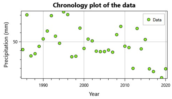
Figure 1. Different year maximum precipitation data distribution in chronology plot.

The data on annual maxima are plotted using a rank-order approach. In order to do this, the data must be arranged from largest to smallest event, with the largest event being assigned a rank of 1 and the smallest event a rank of n. The rank (i) of each event is then used to determine the probability plotting position. Numerous formulas for graphing positions are variations of the general formula

[13, 14]

Where P_i is the exceedance probability for an event of rank I, α is a constant more than or equal to 0 and less than 1, n is the sample size, and i is the event's rank. The calculated plotting positions' fit to a given theoretical probability distribution is determined by the value of α.

Download: Download full-size image

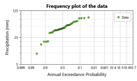
Figure 2. Different year maximum precipitation data distribution in frequency plot.

Plotting positions Weibull (α = 0.0), Median (α = 0.03175), Blom (α = 0.375), Cunnane (α = 0.40), Gringorten (α = 0.44), and Hazen (α = 0.50) all have distinct values for the plotting position parameter α

[14]

. Because it is unbiased for all distributions, the Weibull plotting position parameter (α = 0.0) was used for this particular investigation and is advised as the default option.

After understanding the raw data characteristics, the next step was determining quality of the data through data quality test. Because hydrological data can have errors because of recording devices or observers. Direct data analysis might lead to expensive costs since it overestimates the design discharge or deteriorates any hydraulic infrastructure. For this reason, an outlier test and a standard error test were performed on the chosen station attributes of the data. According to

[15, 16]

the data’s were considered as adequate if the relative standard errors in the data should be less than ten percent (10%). The formula to estimate the relative standard error is:

Relative standard error,

δ_{e}

\frac{S_{e}}{\overset{̅}{p}}

S_e=

\frac{δ_{n - 1}}{\sqrt{N}}

\overset{̅}{p}

\frac{\sum p}{N}

From daily data available, peak annual rainfall was selected and have the following statistical parameters.

Table 2. Statistical parameters of the data.

Parameter	Number of samples, N	Summation, $\sum p$	Average, $\overset{̅}{p}$	Standard deviation, $δ_{n - 1}$
Value	35	1633.8	46.68	18.7

Additionally, some data may fall above or below the threshold because of observer, instrument, or other deterioration that taints the meteorological record. By doing an outlier test on the data, such data were controlled and modified. Data points that drastically deviate from the overall trend are known as outliers. The size of statistical parameters calculated from the data is greatly impacted by the retention or depletion of these outliers

[16]

. Depending on the skewness coefficient, the test was run on logarithmic modified data.

Table 3. Outlier test skewness coefficient range.

Skewness coefficient	> +0.4	< -0.4	Between ± 4
Test for	Higher outliers	Lower outlier	Both high and low outliers

Source:

[17]

The following equations can be used to detect higher and lower outliers:

y_h=

\overset{̅}{y}

+ k_nS_y

y_L=

\overset{̅}{y}

- k_nS_y

Where: y_h and y_L are high and low outlier threshold in log units respectively

k_n = coefficient depends on sample size (for N = 35; k_n= 2.628)

[17]

\overset{̅}{y}

= mean of the data in log unit

S_y= standard deviation in log unit

Table 4. Statistical parameters and analysis of log transformed data.

Parameter	Summation	Mean	Standard deviation	Skewness
Value	56.9566	1.627	0.2094	-1.1394

2.2. Rainfall Data Disaggregation

Given that floods in urban areas typically occur for brief periods of time, drainage systems there were built to withstand shorter rainfall durations. There are few short-term data sources or records available in Ethiopia, and these meteorological data were typically recorded on a daily basis. Therefore, it is vital to identify storm episodes with shorter durations before moving straight into hydrological analysis. The following algorithm is suggested by

[18]

to break down daily rainfall data into shorter time periods:

R_t=

\frac{{t (b + 24)}^{n}}{{(24 (b + t)}^{n}}

*R₂₄

Where R_t = Rainfall of required duration

R₂₄ = Rainfall of 24hr (daily rainfall)

t = Rainfall required duration

b = Coefficients (0.3)

n = Coefficients (0.78 – 1.09)

The results of the daily data were determined to be identical to the disaggregated daily data using n = Coefficients (1.008).

The daily (24-hour) recorded data was divided into shorter durations of 5 minutes, 15 minutes, 30 minutes, 1 hour, 2 hours, 4 hours, 8 hours, 12 hours, 16 hours, 20 hours, and 24 hours using the method given. The statistical parameters for the original and logarithmic change were:

Table 5. Statistical parameters for disaggregated data for each duration.

Duration (min or hr)	5min	15min	30min	1hr	2hr	4hr	8hr	12hr	16hr	20hr	24hr
Mean	10.62	22.14	30.36	37.22	41.88	44.58	45.95	46.36	46.54	46.63	46.68
Standard deviation	4.25	8.87	12.16	14.91	16.78	17.86	18.41	18.57	18.65	18.68	18.70
Skewness	0.20	0.20	0.20	0.20	0.20	0.20	0.20	0.20	0.20	0.20	0.20

Table 6. Statistical parameters for logarithmic disaggregated data for each duration.

Duration (min or hr)	5min	15min	30min	1hr	2hr	4hr	8hr	12hr	16hr	20hr	24hr
Mean	0.98	1.30	1.44	1.53	1.58	1.61	1.62	1.62	1.63	1.63	1.63
Standard deviation	0.21	0.21	0.21	0.21	0.21	0.21	0.21	0.21	0.21	0.21	0.21
Skewness	-1.14	-1.14	-1.14	-1.14	-1.14	-1.14	-1.14	-1.14	-1.14	-1.14	-1.14

2.3. Intensity Duration Frequency (IDF) Curve Development and Distribution Method Selection

Using probability distribution functions, an Intensity Duration (IDF) curve was constructed for the disaggregated precipitation data. To determine the magnitude of maximum rainfall intensities, the most widely used probability distribution function (PDF) is the Gumbel, Normal, Log-Normal, Pearson type-3, Log-Pearson type-3, and General Extreme value Type-1 (General EVT-1). Equation used to determine the approximate size of an occurrence, such as the intensity of rainfall by

[17]

as:

X_T=

\overset{̅}{X}

+ K_T

δ_{n - 1}

Where:

\overset{̅}{X}

= Mean of the sample data =

\frac{\sum X}{N}

δ_{n - 1}

= standard deviation of sample size N =

\sqrt{\frac{\sum ({X - \overset{̅}{X})}^{2}}{N - 1}}

K_T = a frequency factor which is a function of return period T and coefficient of skew Cs

In the event that the variable analyzed is y = log x, then the same method is applied to the statistics for logarithms of the data by using:

y_T=

\overset{̅}{y}

+ K_T

δ_{n - 1}

To calculate the rainfall intensities, the frequency factor, mean, and standard deviation for each probability distribution function (PDF) were calculated (Table 5 and Table 6) and entered into the equation. To fit multiple distributions to the given input data, the maximum likelihood estimation (MLE) method is employed, in accordance with the

[14]

recommendations. Comparing each distribution's Akaike (AIC), Bayesian information criteria (BIC), or Root Mean Square Error (RMSE) can help in model selection. A smaller value denotes a better fit between the distribution and the input data, according to these metrics.

2.4. Calibration and Evaluation of Selected Method with Non-Probability Idf Models

Non-probability IDF models were used to calibrate and assess the IDF value produced by employing a single probability frequency distribution technique that fits the study area station data. The following formulas are used to calculate the rainfall intensities for various return times and durations, according Nwaogazie & Sam (2019):

Sherman equation, I =

\frac{c T^{m}}{t^{a}}

Talbot equation, I =

\frac{c}{b + t}

Power equation, I = c

t^{a}

Where: I= rainfall intensity (mm/hr)

t = Duration (minutes)

T = Return period (years)

c, m, a, and b are regional constants

The Intensity Duration Frequency (IDF) equations were calibrated by the use of non-linear regression analysis. This approach necessitates the use of Excel Solver, a Microsoft Excel optimization methodology for estimating the Intensity Duration Frequency (IDF) models' parameters. This step requires entering the calculated values from the probability distribution function (PDF) into the spreadsheet as an observed intensity along with its duration and return time. For the assumed values of the IDF equation parameters, intensities associated with the IDF equation for each return period and duration were computed.

[19]

recommends Generalized Reduced Gradient (GRG) solver in the equation was used to minimize the sum of squares of the deviation/error between the observed intensity and the anticipated intensity in order to determine the values of the optimal IDF parameters. As a result, the objective function is as follows:

Min SSE =

\sum_{i = 1}^{n} ({I_{obs} - I_{pred})}^{2}

The Sherman quotient-power equation was used to derive IDF models from the Intensity Duration Frequency (IDF) equation. Through an iterative method that yields least square error, the equation is solved to yield an optimal value for the constants c, m, and a for the chosen IDF equation. The results generated using probability distribution method and non-probability IDF models was checked using performance evaluation criteria or performance indicators based on

[20]

recommend acceptable values for coefficient of determination (r²) > 0.60, the Nash–Sutcliffe efficiency (NSE) > 50 and percent bias (PBIAS) ≤ ±15.

Table 7. Equations, ranges, optimal values of statistical performance measures.

Performance indicator	Equation	Range	Optimal value
Coefficient of determination (r²)	${[\frac{\sum_{i = 1}^{n} (O_{i} - \bar{O}) (P_{i} - \bar{P})}{\sqrt{\sum_{i = 1}^{n} {(O_{i} - \bar{O})}^{2}} \sqrt{\sum_{i = 1}^{n} ({(P_{i} - \bar{P})}^{2})}}]}^{2}$	0.0 to 1.0	1
The Nash–Sutcliffe efficiency (NSE)	$1 - \frac{\sum_{i = 1}^{n} {(O_{i} - P_{i})}^{2}}{\sum_{i = 1}^{n} {(O_{i} - \bar{O})}^{2}}$	-∞ to 1.0	1
Percent bias (PBIAS)	$\frac{\sum_{i = 1}^{n} O_{i} - P_{i}}{\sum_{}^{ni = 1} O_{i}} X 100$	-∞ to ∞	0

Source:

[20]

3. Results and Discussion

The data's relative standard error value, as determined by the data quality test, is 6.77%, falling within the allowed limit of 10%. Additionally, because the skewness coefficient was -1.134, which is less than -0.4, the statistical parameter skewness of the data instructs to compute the outlier test at a lower threshold. According to the test, the lower threshold value was 11.94 mm, which is higher than the 9.5 mm value of the raw data that was obtained.

Download: Download full-size image

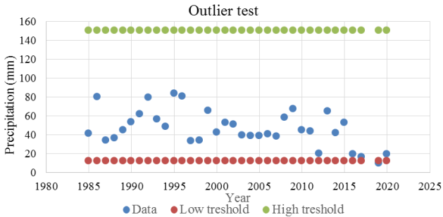
Figure 3. Outlier test graph.

The red dotted line on the graph above the data below indicates data that is outside the lower threshold and is eliminated for additional Intensity Duration Frequency (IDF) curve development analysis. An intensity duration frequency curve was created for several distribution techniques based on the decomposed data. The frequency and cumulative distribution plot that results from using various distribution methods looks like this:

Download: Download full-size image

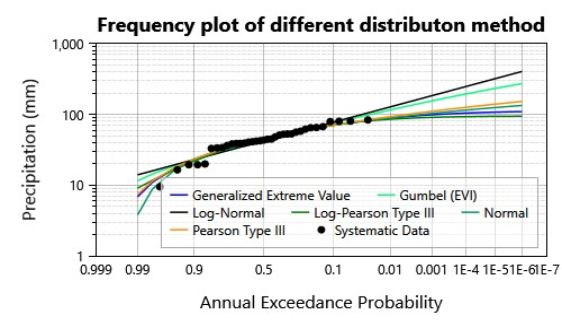
Figure 4. Different distribution method frequency plot in comparison with the station data.

Download: Download full-size image

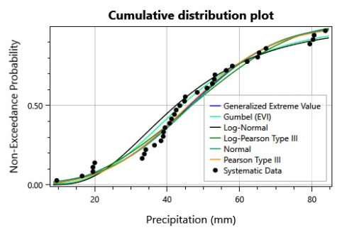
Figure 5. Cumulative distribution plot of different probability distribution methods.

Table 8. The results of different comparison criteria as stated by

[14]

Distribution	AIC	BIC	RMSE
Generalized Extreme Value	309.38	313.27	3.29
Gumbel (EVI)	310.07	312.81	4.01
Log-Normal	313.93	316.66	5.33
Log-Pearson Type III	308.8	312.69	3.38
Normal	307.69	310.42	3.36
Pearson Type III	309.77	313.67	3.23

The AIC and BIC values of a normal distribution are smaller, while the RMSE value is comparatively low. Consequently, this distribution was thought to be a fitting technique for the study region station data. Since, in all cases of stated probability distribution method the formula is similar in determining approximate values of magnitude of an event like rainfall intensity. The only difference is the frequency factor, and for this case (normal distribution method) the frequency factor depends mainly on the return periods. Based on the formula given in

[17]

rainfall intensity values for different duration and return period was calculated.

Table 9. Rainfall intensity for the selected distribution method (normal distribution).

Duration (min)	Return period
Duration (min)	2	5	10	25	50	100	1000
5	127.42	170.37	192.85	216.80	232.28	246.19	285.18
15	88.58	118.44	134.06	150.72	161.47	171.15	198.25
30	60.72	81.18	91.89	103.31	110.68	117.31	135.89
60	37.22	49.76	56.33	63.33	67.85	71.91	83.30
120	20.94	28.00	31.69	35.63	38.17	40.46	46.87
240	11.14	14.90	16.87	18.96	20.32	21.53	24.94
480	5.74	7.68	8.69	9.77	10.47	11.10	12.85
720	3.86	5.17	5.85	6.57	7.04	7.47	8.65
960	2.91	3.89	4.40	4.95	5.30	5.62	6.51
1200	2.33	3.12	3.53	3.97	4.25	4.51	5.22
1440	1.94	2.60	2.94	3.31	3.55	3.76	4.35

Download: Download full-size image

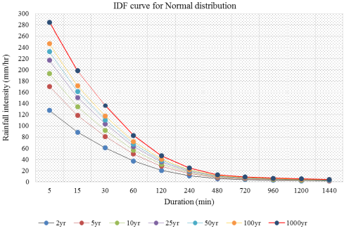
Figure 6. Intensity Duration Frequency curve for the selected distribution method (normal distribution).

Using Excel Solver for the Intensity Duration Frequency (IDF) equation (Sherman quotient-power equation), the optimum values for constants c, m, and a become 362.55, 0.1045, and 0.53 respectively, which yield the minimum sum square error during calibration of the IDF generated using the Normal probability distribution method. The matching equation is now:

Sherman equation, I =

\frac{362.55 T^{0.1045}}{t^{0.53}}

Table 10. The resulting intensity value generated using excel solver using Sherman equation.

Duration (min)	Return period
Duration (min)	2	5	10	25	50	100	1000
5	166.01	182.69	196.41	216.14	232.37	249.83	317.78
15	92.70	102.02	109.68	120.70	129.76	139.51	177.45
30	64.19	70.64	75.94	83.57	89.85	96.60	122.87
60	44.44	48.91	52.58	57.86	62.21	66.88	85.07
120	30.77	33.86	36.41	40.06	43.07	46.31	58.90
240	21.31	23.45	25.21	27.74	29.82	32.06	40.78
480	14.75	16.23	17.45	19.21	20.65	22.20	28.24
720	11.90	13.09	14.08	15.49	16.65	17.90	22.77
960	10.21	11.24	12.08	13.30	14.30	15.37	19.55
1200	9.07	9.99	10.74	11.81	12.70	13.66	17.37
1440	8.24	9.07	9.75	10.73	11.53	12.40	15.77

The probability distribution function and non-probability IDF models are used to generate the performance indices parameter of the IDF. The result becomes:

Table 11. Performance index result.

Performance index	Value
R²	0.96
NSE	0.964
PBIAS	-6.35%

The performance index requirements were found to be within an acceptable range based on

[20]

. Consequently, the distribution approach that best suited the research area station data was the Normal probability distribution method.

Download: Download full-size image

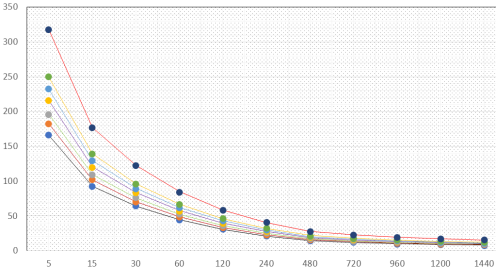
Figure 7. Calibrated Intensity Duration Frequency curve for the selected distribution method.

4. Conclusion

Finding row data is important for hydrologic analysis, but so is the quality of the data that is accessible. Prior to further application and modeling, any researcher must first thoroughly grasp the raw data and assess its quality. In particular, shorter duration rainfall intensity is required for urban drainage models since urban floods occur over shorter periods of time. This was accomplished by breaking down the 24-hour rainfall into shorter periods using a formula developed by the Ethiopia Road Authority (ERA). The level of intensity Time frame After analyzing the frequency curves of several distribution techniques, the normal distribution was found to best fit the chosen station. Furthermore, there is a positive correlation between the comparison result and the non-probability IDF model. Therefore, while planning, constructing, and implementing hydraulic structures for the designated site, rainfall intensity values produced by the normal distribution approach can be applied. Additionally, the outcome demonstrates that researchers can use the distribution mechanism that was developed to construct any hydrologic model.

Abbreviations

AACRA	Addis Ababa City Road Authority
AIC	Akaike Information Criteria
BIC	Bayesian Information Criteria
ERA	Ethiopia Road Authority
EVT	Extreme Value Type
GRG	Generalized Reduced Gradient
IDF	Intensity Duration Curve
NMA	National Meteorology Agency
NSE	Nash-Sutcliffe Efficiency
PBIAS	Percent Bias
PDF	Probability Distribution Function
RMSE	Root Mean Square Error

Acknowledgments

The authors acknowledge Ethiopian Ministry of Water, Irrigation and Energy and the National Metrological Agency for providing the necessary data.

Funding

The research has no any funding organization.

Data Availability Statement

Data used in this research are available upon request.

Conflicts of Interest

The authors declare no conflicts of interest.

References

[1]	AACRA, “Urban Road Drainage Precipitation,” in Addis Ababa City Road Authority Drainage Design Manual, Addis Ababa, Ethiopia: Addis Ababa City Road Authority, Addis Ababa; Ethiopia, 2004.
[2]	C. C. Mbajiorgu, “Development of Intensity Duration Frequency (IDF) Curve for Parts of Eastern Catchments Using Modern Arcview GIS Model,” no. January 2012, 2015.
[3]	T. Vischel and G. Panthou, “Technical notes on Intensity-duration-frequency curves for the city of Ouagadougou : A tool for helping with the dimensioning of hydraulic structures,” pp. 1–6, 2018.
[4]	F. De Paola, M. Giugni, M. E. Topa, and E. Bucchignani, “Intensity-Duration-Frequency (IDF) rainfall curves, for data series and climate projection in African cities,” vol. 3, no. 1, pp. 1–18, 2014, https://doi.org/10.1186/2193-1801-3-133
[5]	A. Shrestha, M. S. Babel, S. Weesakul, and Z. Vojinovic, “Developing Intensity – Duration – Frequency (IDF) Curves under Climate Change Uncertainty : The Case,” 2017, https://doi.org/10.3390/w9020145
[6]	T. Amona and W. E. Worajo, “Developing Maximum Intensity Duration Frequency (IDF) Curve to WolaitaSodo City, Ethiopia,” vol. 24, no. 5, pp. 62–76, 2022.
[7]	V. Basumatary and B. S. Sil, “Generation of Rainfall Intensity-Duration-Frequency curves for the Barak River Basin,” vol. 6, 2016.
[8]	G. Ena et al., “Case Study : Depth-Duration Ratio in a Semi-Arid Zone in Mexico,” MDPI, 2020.
[9]	S. T. Thanh and A. H. Xuan, “Deriving of Intensity- Duration- Frequency (IDF) curves for precipitation at Hanoi, Vietnam,” E3 S Web Conf., vol. 403, 2023, https://doi.org/10.1051/e3sconf/202340306002
[10]	R. M. Wambua, “Estimating Rainfall Intensity-Duration-Frequency (Idf) Curves For A Tropical River Basin,” Int. J. Adv. Res. Publ., vol. 3, no. 4, pp. 99–106, 2019.
[11]	Y. Sun, D. Wendi, D. E. Kim, and S. Y. Liong, “Deriving intensity–duration–frequency (IDF) curves using downscaled in situ rainfall assimilated with remote sensing data,” Geosci. Lett., vol. 6, no. 1, 2019, https://doi.org/10.1186/s40562-019-0147-x
[12]	H. Van De Vyver, G. R. Demarée, H. Van De Vyver, and G. R. Demarée, “Construction of Intensity – Duration – Frequency (IDF) curves for precipitation at Lubumbashi, Congo, under the hypothesis of inadequate data Construction of Intensity – Duration – Frequency (IDF) curves for precipitation at Lubumbashi, Congo, und,” vol. 6667, no. May, 2010, https://doi.org/10.1080/02626661003747390.
[13]	D. A. Jones, “Plotting positions via maximum-likelihood for a non-standard situation,” Hydrology and Earth System Sciences, vol. 1, no. 2. pp. 357–366, 1997. https://doi.org/10.5194/hess-1-357-1997
[14]	U.S. Army Corps of Engineers (USACE), “RMC-BestFit Quick Start Guide,” p. 99, 2020, [Online]. Available: https://www.iwrlibrary.us/#/document/f1767e9f-714d-43b7-cf74-ed1bd65f9dd9
[15]	H. M. Raghunath, Hydrology Principles, Analysis, and Design, Revised Se. New Delhi: New Age International, 2006.
[16]	K. Subramanya, “Engineering Hydrology,” 4th ed., New Delhi; India: McGraw Hill Education, 2013.
[17]	V. Te Chow, D. R. Maidment, and L. W. Mays, Applied Hydrology, McGRAW-HIL. McGraw-Hill, 1988.
[18]	ERA, “Drainage design manual,” in Ethiopia Road Authority Drainage Design Manual; Ethiopia, Addis Ababa, 2013.
[19]	I. L. Nwaogazie and M. G. Sam, “Probability and non-probability rainfall intensity- duration-frequency modeling for Port-Harcourt metropolis, Nigeria,” vol. 3, no. 1, 2019, https://doi.org/10.15406/ijh.2019.03.00164
[20]	D. Moriasi, M. Gitau, N. Pai, and P. Daggupati, “Hydrologic and Water Quality Models: Performance Measures and Evaluation Criteria,” no. December, 2015, https://doi.org/10.13031/trans.58.10715

Cite This Article

Plain Text BibTeX RIS

APA Style

Agza, M. D., Assefa, A. L., Legeta, B. W. (2025). Advancement of Intensity Duration Frequency (IDF) Curve Through Possible Probability Distribution Method Using Disaggregated Precipitation Data; The Case of Wolkite, Ethiopia. American Journal of Water Science and Engineering, 11(2), 30-39. https://doi.org/10.11648/j.ajwse.20251102.13

Copy | Download

ACS Style

Agza, M. D.; Assefa, A. L.; Legeta, B. W. Advancement of Intensity Duration Frequency (IDF) Curve Through Possible Probability Distribution Method Using Disaggregated Precipitation Data; The Case of Wolkite, Ethiopia. Am. J. Water Sci. Eng. 2025, 11(2), 30-39. doi: 10.11648/j.ajwse.20251102.13

Copy | Download

AMA Style

Agza MD, Assefa AL, Legeta BW. Advancement of Intensity Duration Frequency (IDF) Curve Through Possible Probability Distribution Method Using Disaggregated Precipitation Data; The Case of Wolkite, Ethiopia. Am J Water Sci Eng. 2025;11(2):30-39. doi: 10.11648/j.ajwse.20251102.13

Copy | Download

@article{10.11648/j.ajwse.20251102.13,
  author = {Mezen Desse Agza and Andwelam Leta Assefa and Beyene Wolde Legeta},
  title = {Advancement of Intensity Duration Frequency (IDF) Curve Through Possible Probability Distribution Method Using Disaggregated Precipitation Data; The Case of Wolkite, Ethiopia
},
  journal = {American Journal of Water Science and Engineering},
  volume = {11},
  number = {2},
  pages = {30-39},
  doi = {10.11648/j.ajwse.20251102.13},
  url = {https://doi.org/10.11648/j.ajwse.20251102.13},
  eprint = {https://article.sciencepublishinggroup.com/pdf/10.11648.j.ajwse.20251102.13},
  abstract = {Rainfall is one of the key inputs for surface water resources and groundwater recharges. This rainfall is recorded in depth format (mm or in) using a rain gauge in the gauging station. Some models need this rainfall record in intensity format (example, mm/hr or in/hr). In addition, design discharge, especially flood-related structures, requires extreme rainfall intensity values. In Ethiopia availability of on hand rainfall intensity data in shortest duration is in scarce and the same for the selected area called Wolkite. Therefore, this study aims in developing Intensity Duration Frequency curve through probability distribution methods using disaggregated data that fits the study area. For this purpose, six distribution methods, namely, general extreme value I, Gumbel, normal, log-normal, Pearson, and log-Pearson were examined based on different comparison criteria. Normal distribution method found to be the best method that fits the data applied and Intensity duration curve was developed using this method. Finally, the developed Intensity Duration Frequency curve was calibrated and evaluated with Non-Probability Intensity Duration Frequency Models and results a Performance indicator value of Coefficient of determination (R2), Nash-Sutcliffe efficiency (NSE) and Percent bias (PBIAS) of 0.96, 0.964, and -6.35% which are in acceptable ranges. Therefore, the derived Intensity Duration Frequency values were possible to apply in developments of any urban and water related structure for required duration specifically in Wolkite town. Also, the research is applied as a guideline in areas where availability of rainfall intensities of shortest duration is in scarce.
},
 year = {2025}
}

Copy | Download

TY  - JOUR
T1  - Advancement of Intensity Duration Frequency (IDF) Curve Through Possible Probability Distribution Method Using Disaggregated Precipitation Data; The Case of Wolkite, Ethiopia

AU  - Mezen Desse Agza
AU  - Andwelam Leta Assefa
AU  - Beyene Wolde Legeta
Y1  - 2025/06/25
PY  - 2025
N1  - https://doi.org/10.11648/j.ajwse.20251102.13
DO  - 10.11648/j.ajwse.20251102.13
T2  - American Journal of Water Science and Engineering
JF  - American Journal of Water Science and Engineering
JO  - American Journal of Water Science and Engineering
SP  - 30
EP  - 39
PB  - Science Publishing Group
SN  - 2575-1875
UR  - https://doi.org/10.11648/j.ajwse.20251102.13
AB  - Rainfall is one of the key inputs for surface water resources and groundwater recharges. This rainfall is recorded in depth format (mm or in) using a rain gauge in the gauging station. Some models need this rainfall record in intensity format (example, mm/hr or in/hr). In addition, design discharge, especially flood-related structures, requires extreme rainfall intensity values. In Ethiopia availability of on hand rainfall intensity data in shortest duration is in scarce and the same for the selected area called Wolkite. Therefore, this study aims in developing Intensity Duration Frequency curve through probability distribution methods using disaggregated data that fits the study area. For this purpose, six distribution methods, namely, general extreme value I, Gumbel, normal, log-normal, Pearson, and log-Pearson were examined based on different comparison criteria. Normal distribution method found to be the best method that fits the data applied and Intensity duration curve was developed using this method. Finally, the developed Intensity Duration Frequency curve was calibrated and evaluated with Non-Probability Intensity Duration Frequency Models and results a Performance indicator value of Coefficient of determination (R2), Nash-Sutcliffe efficiency (NSE) and Percent bias (PBIAS) of 0.96, 0.964, and -6.35% which are in acceptable ranges. Therefore, the derived Intensity Duration Frequency values were possible to apply in developments of any urban and water related structure for required duration specifically in Wolkite town. Also, the research is applied as a guideline in areas where availability of rainfall intensities of shortest duration is in scarce.

VL  - 11
IS  - 2
ER  -

Copy | Download

Author Information

Mezen Desse Agza

Department of Hydraulic and Water Resource Engineering, Wolkite University, Wolkite, Ethiopia

Contact Email

http://orcid.org/0009-0008-0026-3421
Andwelam Leta Assefa

Department of Hydraulic and Water Resource Engineering, Wolkite University, Wolkite, Ethiopia

http://orcid.org/0009-0007-2945-1912
Beyene Wolde Legeta

Construction Project Office, Wolkite University, Wolkite, Ethiopia

http://orcid.org/0009-0006-9749-5434

Download PDF

Plain Text BibTeX RIS

APA Style

Agza, M. D., Assefa, A. L., Legeta, B. W. (2025). Advancement of Intensity Duration Frequency (IDF) Curve Through Possible Probability Distribution Method Using Disaggregated Precipitation Data; The Case of Wolkite, Ethiopia. American Journal of Water Science and Engineering, 11(2), 30-39. https://doi.org/10.11648/j.ajwse.20251102.13

Copy | Download

ACS Style

Agza, M. D.; Assefa, A. L.; Legeta, B. W. Advancement of Intensity Duration Frequency (IDF) Curve Through Possible Probability Distribution Method Using Disaggregated Precipitation Data; The Case of Wolkite, Ethiopia. Am. J. Water Sci. Eng. 2025, 11(2), 30-39. doi: 10.11648/j.ajwse.20251102.13

Copy | Download

AMA Style

Agza MD, Assefa AL, Legeta BW. Advancement of Intensity Duration Frequency (IDF) Curve Through Possible Probability Distribution Method Using Disaggregated Precipitation Data; The Case of Wolkite, Ethiopia. Am J Water Sci Eng. 2025;11(2):30-39. doi: 10.11648/j.ajwse.20251102.13

Copy | Download

@article{10.11648/j.ajwse.20251102.13,
  author = {Mezen Desse Agza and Andwelam Leta Assefa and Beyene Wolde Legeta},
  title = {Advancement of Intensity Duration Frequency (IDF) Curve Through Possible Probability Distribution Method Using Disaggregated Precipitation Data; The Case of Wolkite, Ethiopia
},
  journal = {American Journal of Water Science and Engineering},
  volume = {11},
  number = {2},
  pages = {30-39},
  doi = {10.11648/j.ajwse.20251102.13},
  url = {https://doi.org/10.11648/j.ajwse.20251102.13},
  eprint = {https://article.sciencepublishinggroup.com/pdf/10.11648.j.ajwse.20251102.13},
  abstract = {Rainfall is one of the key inputs for surface water resources and groundwater recharges. This rainfall is recorded in depth format (mm or in) using a rain gauge in the gauging station. Some models need this rainfall record in intensity format (example, mm/hr or in/hr). In addition, design discharge, especially flood-related structures, requires extreme rainfall intensity values. In Ethiopia availability of on hand rainfall intensity data in shortest duration is in scarce and the same for the selected area called Wolkite. Therefore, this study aims in developing Intensity Duration Frequency curve through probability distribution methods using disaggregated data that fits the study area. For this purpose, six distribution methods, namely, general extreme value I, Gumbel, normal, log-normal, Pearson, and log-Pearson were examined based on different comparison criteria. Normal distribution method found to be the best method that fits the data applied and Intensity duration curve was developed using this method. Finally, the developed Intensity Duration Frequency curve was calibrated and evaluated with Non-Probability Intensity Duration Frequency Models and results a Performance indicator value of Coefficient of determination (R2), Nash-Sutcliffe efficiency (NSE) and Percent bias (PBIAS) of 0.96, 0.964, and -6.35% which are in acceptable ranges. Therefore, the derived Intensity Duration Frequency values were possible to apply in developments of any urban and water related structure for required duration specifically in Wolkite town. Also, the research is applied as a guideline in areas where availability of rainfall intensities of shortest duration is in scarce.
},
 year = {2025}
}

Copy | Download

TY  - JOUR
T1  - Advancement of Intensity Duration Frequency (IDF) Curve Through Possible Probability Distribution Method Using Disaggregated Precipitation Data; The Case of Wolkite, Ethiopia

AU  - Mezen Desse Agza
AU  - Andwelam Leta Assefa
AU  - Beyene Wolde Legeta
Y1  - 2025/06/25
PY  - 2025
N1  - https://doi.org/10.11648/j.ajwse.20251102.13
DO  - 10.11648/j.ajwse.20251102.13
T2  - American Journal of Water Science and Engineering
JF  - American Journal of Water Science and Engineering
JO  - American Journal of Water Science and Engineering
SP  - 30
EP  - 39
PB  - Science Publishing Group
SN  - 2575-1875
UR  - https://doi.org/10.11648/j.ajwse.20251102.13
AB  - Rainfall is one of the key inputs for surface water resources and groundwater recharges. This rainfall is recorded in depth format (mm or in) using a rain gauge in the gauging station. Some models need this rainfall record in intensity format (example, mm/hr or in/hr). In addition, design discharge, especially flood-related structures, requires extreme rainfall intensity values. In Ethiopia availability of on hand rainfall intensity data in shortest duration is in scarce and the same for the selected area called Wolkite. Therefore, this study aims in developing Intensity Duration Frequency curve through probability distribution methods using disaggregated data that fits the study area. For this purpose, six distribution methods, namely, general extreme value I, Gumbel, normal, log-normal, Pearson, and log-Pearson were examined based on different comparison criteria. Normal distribution method found to be the best method that fits the data applied and Intensity duration curve was developed using this method. Finally, the developed Intensity Duration Frequency curve was calibrated and evaluated with Non-Probability Intensity Duration Frequency Models and results a Performance indicator value of Coefficient of determination (R2), Nash-Sutcliffe efficiency (NSE) and Percent bias (PBIAS) of 0.96, 0.964, and -6.35% which are in acceptable ranges. Therefore, the derived Intensity Duration Frequency values were possible to apply in developments of any urban and water related structure for required duration specifically in Wolkite town. Also, the research is applied as a guideline in areas where availability of rainfall intensities of shortest duration is in scarce.

VL  - 11
IS  - 2
ER  -

Copy | Download