An Explainable AI Framework for Neonatal Mortality Risk Prediction in Kenya: Enhancing Clinical Decisions with Machine Learning

Victor Wandera Lumumba; Dennis Kariuki Muriithi; Elizabeth Wambui Njoroge; Amos Kipkorir Langat; Edson Mwebesa; Maureen Ambasa Wanyama

doi:doi:10.11648/j.bsi.20251003.12

Research Article |

| Peer-Reviewed

An Explainable AI Framework for Neonatal Mortality Risk Prediction in Kenya: Enhancing Clinical Decisions with Machine Learning

Victor Wandera Lumumba^*

, Dennis Kariuki Muriithi

, Elizabeth Wambui Njoroge

, Amos Kipkorir Langat

, Edson Mwebesa

, Maureen Ambasa Wanyama

Published in Biomedical Statistics and Informatics (Volume 10, Issue 3)

Received: 21 August 2025 Accepted: 30 August 2025 Published: 30 September 2025

Views: Downloads:

Download PDF

Share This Article

Twitter
Linked In
Facebook

Abstract

Neonatal mortality remains a critical public health challenge in Kenya, with a rate of 21 per 1,000 live births—well above the SDG 3.2 target. While machine learning (ML) offers potential for risk prediction, most models lack transparency and clinical interpretability, limiting their adoption in low-resource settings. This study presents an explainable AI (XAI) framework for predicting neonatal mortality using Kenya Demographic and Health Survey (KDHS) data (N = 2,000), with a focus on model accuracy, fairness, and clinical relevance. Six ML models—Logistic Regression (LR), KNN, SVM, Naïve Bayes, Random Forest, and XG-Boost—were trained and evaluated using in-sample, out-of-sample, and balanced datasets, with performance assessed via AUC, F1-score, sensitivity, specificity, and Cohen’s Kappa. To address class imbalance and enhance generalizability, synthetic oversampling and rigorous cross-validation were applied. Post-balancing, LR achieved optimal performance (AUC = 1.0, κ = 0.98, F1 = 0.987), with SVM (AUC = 0.995) and XG-Boost (AUC = 0.982) also showing higher performance. SHAP and model breakdown analyses identified Apgar scores (at 1st and 5th minutes), birth weight, maternal health, and prenatal visit frequency as key predictors. Fairness assessments across socioeconomic subgroups indicated minimal bias (DIR > 0.8). The integration of XAI enhances transparency, supports clinician trust, and enables equitable decision-making. This framework bridges the gap between predictive accuracy and clinical usability, offering a scalable tool for early intervention. Policy recommendations include embedding this XAI-enhanced model into antenatal care systems to support evidence-based decisions and accelerate progress toward neonatal survival goals in resource-limited settings.

Published in	Biomedical Statistics and Informatics (Volume 10, Issue 3)
DOI	10.11648/j.bsi.20251003.12
Page(s)	64-83
Creative Commons	This is an Open Access article, distributed under the terms of the Creative Commons Attribution 4.0 International License (http://creativecommons.org/licenses/by/4.0/), which permits unrestricted use, distribution and reproduction in any medium or format, provided the original work is properly cited.
Copyright	Copyright © The Author(s), 2025. Published by Science Publishing Group

Keywords

Explainable Artificial Intelligence (XAI), Neonatal Mortality, Machine Learning, Predictive Modelling, Health Belief Model, Calibration

1. Introduction

Neonatal mortality remains one of the most pressing challenges in global health. Worldwide, approximately 2.3 million newborns died in the first month of life in 2022, accounting for nearly 47% of all under-five deaths

[1]

. While this represents a decline from about 5 million neonatal deaths in 1990, progress has slowed in recent years

[2]

The burden is disproportionately concentrated in low- and middle-income countries (LMICs), with Sub-Saharan Africa (SSA) and South Asia recording the highest neonatal death rates in 2023 at 26 and 22 per 1,000 live births, respectively

[3]

. A newborn in SSA is over ten times more likely to die within the first month compared to one in high-income settings, with global disparities reaching as high as 65-fold between the worst-off and safest countries

[4]

. In Kenya, despite sustained efforts over the past two decades, neonatal mortality remains a significant health priority

[5]

. According to the 2023 Kenya Vital Statistics Report, the neonatal mortality rate declined from 33 to 21 per 1,000 live births between 2003 and 2022; however, it remains far above the Sustainable Development Goal (SDG) 3.2 target of 12 per 1,000 live births by 2030

[6]

. Neonatal deaths account for 66% of infant deaths and 51% of under-five deaths, highlighting their outsized contribution to child mortality

[7]

. To accelerate progress toward SDG 3, innovative strategies tailored to resource-limited environments are urgently needed

[8]

. Machine learning (ML) and artificial intelligence (AI) have emerged as promising tools for predicting neonatal mortality risk and supporting timely interventions

[9]

. Evidence suggests that ML can outperform or complement traditional statistical methods in stratifying risk. For example, a 2024 multi-centre Neonatal Intensive Care Unit (NICU) modelling competition reported that a simple logistic regression model outperformed more complex methods, including deep learning, in predicting mortality

[10]

. A 2021 systematic review identified 11 studies applying ML to neonatal mortality prediction across diverse populations, using algorithms such as neural networks, random forests, and logistic regression with between 3 and 60+ features

[11]

. Reported performance ranged widely (AUC 58-97%), but most studies lacked external validation or calibration, revealing methodological limitations in this emerging field. In LMICs, research is growing but remains limited. For instance, ML models trained on Demographic and Health Survey (DHS) data across 10 SSA countries successfully identified maternal risk of neonatal death

[12]

. In Ethiopia, an ensemble CatBoost model achieved over 97% AUC in predicting neonatal deaths, identifying actionable factors such as lack of BCG vaccination, neonatal illness, insufficient maternal prenatal care, and larger numbers of young children in the household

[13]

. These findings illustrate the potential of ML to uncover context-relevant determinants of neonatal survival. However, most models have been evaluated in retrospective or tertiary care datasets, with few applied in routine clinical contexts in Africa

[14]

Despite promising predictive performance, most neonatal mortality models remain “black boxes,” offering limited transparency into their decision-making

[15]

. Clinicians require interpretable outputs—such as identifying low birth weight, maternal comorbidities, or Apgar scores—as key drivers of prediction to trust and act upon AI recommendations

[16]

. Without explainability, even accurate models may go unused or be misapplied. A 2021 review found that most neonatal mortality prediction studies reported accuracy metrics but did not apply explainability techniques, such as SHapley Additive exPlanations (SHAP) or Local Interpretable Model-Agnostic Explanations (LIME), or decision rules

[17]

. This lack of interpretability is a major barrier to adoption in clinical practice.

Explainable AI (XAI) addresses this gap by coupling predictions with human-friendly explanations. Techniques such as SHAP, feature importance rankings, and model breakdown analyses can clarify whether variables such as gestational age, maternal comorbidities, or breastfeeding practices most strongly influenced risk predictions, enabling clinicians to align model reasoning with clinical experience

[18, 19]

. In neonatal sepsis, XAI frameworks such as LIME and DALEX have been utilized to interpret deep learning models for non-technical healthcare providers

[20]

. In resource-constrained African contexts, the need for explainability is especially critical: a well-tuned, transparent ML model can identify high-risk neonates early and prompt timely interventions—such as feeding support, intensified monitoring, or antibiotics—that are proven to reduce mortality

[21, 22]

. The successful deployment of AI-enabled fetal monitoring in Malawi, which reduced stillbirths and neonatal deaths by 82%, underscores the transformative potential of context-sensitive, explainable AI tools

[23]

. Yet prediction alone is insufficient. Responsible clinical deployment requires robust calibration, external validation, subgroup fairness analyses, and integration into clinician workflows

[24, 25]

. Less than half of the published neonatal mortality models report calibration, and only 18% undergo external validation

[26]

, which undermines their clinical reliability and validity. Moreover, few models explicitly evaluate fairness across subgroups, such as sex or socioeconomic status, thereby risking the reinforcement of health inequities

[27]

To address these challenges, this study integrates the Health Belief Model, which emphasizes action when threats are recognized and the benefits of prevention are clear, with Predictive Analytics Theory, which stresses that data-driven insights must be transparent and user-centered (16). Grounded in these frameworks, we propose a machine learning framework that combines predictive accuracy with explainability, contextual relevance, and stakeholder engagement. Specifically, we will (i) develop and compare multiple ML models—logistic regression, k-nearest neighbors, Support vector machines, Naïve bayes, random forests, gradient boosting—using Kenya DHS data; (ii) conduct rigorous internal and external validation, including calibration and subgroup fairness assessments; (iii) embed XAI methods such as SHAP, feature importance, and model breakdowns to enhance interpretability; and (iv) co-design the system with neonatologists, nurses, and data scientists to optimize usability and integration into clinical workflows. By consolidating evidence on explainable AI in neonatal mortality prediction and applying it to the Kenyan context, this study aims to bridge the gap between algorithmic accuracy and actionable clinical intelligence. Ultimately, the framework aims to support clinicians in making timely, evidence-informed decisions, strengthen trust in AI, and contribute to global efforts to reduce neonatal mortality by 2030.

Table 1. Overview of Prior Studies Applying Statistical and Machine Learning Models for Neonatal/Child Mortality.

Study (year)	Setting/data	Model(s)	Outcome	Performance (AUC / C-index)	XAI used?	External validation?	LMIC focus?
Batista et al. 2021 (BMC Pediatrics)	São Paulo, Brazil birth registry (SINASC+SIM), 2012-2017	Gradient boosting, RF, XGB, SVM, LR	Neonatal death (≤28 days)	AUC ≈0.97 overall; with only 5 WHO variables, AUC ≈0.91 (reported by study team in talk materials	Yes—SHAP + feature importance discussed	Internal split; no true external geo-temporal validation reported	Yes
Beluzo et al. 2020 (medRxiv)	São Paulo, Brazil (SPNeoDeath)	SVM, XGBoost, LR, RF	Neonatal death	Average AUC ≈0.96 across models (best models)	Mentions model interpretability; SHAP used in the related slide deck	Internal validation; no external cohort	Yes
Mulagha-Maganga et al. 2024 (JHPN)	Malawi DHS 2015/16	Survival models (e.g., parametric/Cox)	Time to death < 5y	Survival outputs (HRs); AUC not reported	No (classical covariate effects)	Not reported	Yes
Daniel, Onyango & Sarguta 2021 (IJERPH)	Kenya (KDHS)	Bayesian spatial survival model (shared frailty)	Under-five mortality	Survival outputs (HRs/spatial effects); AUC not reported	Partial (spatial effect maps, not XAI)	Not reported	Yes
Wanjohi & Muriithi 2020 (IJDSA)	Kenya	Regression/survival modelling of infant & child mortality covariates	Infant/child mortality	Classical fit metrics; AUC not reported	No	Not reported	Yes
Starnes et al. 2023 (BMJ Open)	Migori County, Kenya (household survey)	Regression models (risk factors)	Child mortality	Effect estimates; no AUC (not an ML study)	No	Not applicable	Yes
Kimani-Murage et al. 2014 (Health & Place)	Kenya (urban slum vs non-slum)	Time-trend and regression analyses	Child mortality trends	No AUC	No	Not applicable	Yes
Otieno, Kosgei & Owuor 2023 (Biomed. Stats & Informatics)	Kenya (KDHS 2014)	Multilevel models	Child mortality determinants	Fit stats: AUC not reported	No	Not reported	Yes
Mwambire & Orowe 2021 (Applied Mathematical Sciences)	Kenya (KDHS)	Multilevel modelling	Child mortality	Fit stats: AUC not reported	No	Not reported	Yes
Oleribe et al. 2019 (IJGM)	Sub-Saharan Africa (review/commentary)	—	Health-system challenges	—	—	—	Yes (context)

As shown in Table 1, while several studies have applied machine learning to neonatal mortality prediction, critical gaps persist, particularly in model interpretability, external validation, and fairness. Only a minority incorporate explainable AI (XAI) techniques, and fewer than 20% undergo external validation, limiting clinical trust and generalizability. Our framework directly addresses these limitations by integrating SHAP-based interpretability, rigorous internal validation using repeated cross-validation, and post-hoc fairness assessments across key demographic subgroups. Furthermore, by leveraging nationally representative KDHS data and co-designing the system with clinicians, we enhance both the contextual relevance and practical deployability of the model in resource-limited settings such as Kenya.

2. Research Methods and Materials

2.1. Research Design

This study employed a quantitative research design to develop and evaluate explainable machine learning models for predicting the risk of neonatal mortality. Secondary data from the Kenya Demographic and Health Survey (KDHS) were analysed using six supervised algorithms: Logistic Regression (benchmark model), K-Nearest Neighbours (KNN), Support Vector Machines (SVM), Naïve Bayes, Random Forests, and Extreme Gradient Boosting (XGBoost). Model training incorporated internal and external validation, calibration, and subgroup fairness assessments, with explainable AI techniques applied to enhance interpretability and clinical applicability.

2.2. Data Collection

The study utilised secondary data obtained from the Kenya Demographic and Health Survey (KDHS), a nationally representative dataset conducted by the Kenya National Bureau of Statistics in collaboration with international partners. The KDHS provides detailed information on maternal, neonatal, and child health indicators, as well as socioeconomic characteristics and household demographics. Data were accessed through the DHS Program with prior authorisation. For this study, relevant variables associated with neonatal outcomes were extracted, cleaned, and preprocessed to ensure completeness, accuracy, and suitability for machine learning analysis.

2.3. Data Analysis

Data analysis involved preprocessing, exploratory statistics, and supervised machine learning modelling. Key maternal, healthcare, infant, and socioeconomic predictors were used to train six algorithms: Logistic Regression, KNN, SVM, Naïve Bayes, Random Forest, and XGBoost. The outcome variable was neonatal mortality (1 = died, 0 = survived). Missing values were imputed, categorical variables were encoded, and numerical variables were standardized. Model evaluation utilized accuracy, sensitivity, specificity, AUC-ROC, and calibration metrics, as well as explainable AI (XAI) methods, including SHAP values and feature importance, to enhance interpretability.

2.3.1. Data Partition and Control Validation

Let the labelled dataset be

D = {(x_{i}, y_{i})}_{i = 1}^{N}, x_{i} \in R^{p}, y_{i} \in {0, 1} .

(1)

Let

N_{c} = \sum_{i = 1}^{N} 1 (y_{i} = c)

and

π_{c} = N_{c} / N

be class counts and priors for

c \in {0, 1}

I. Stratified 70/30 Hold-Out Split

We construct index sets

I = {1, \dots, N}

I_{tr}

(train) and

I_{te}

(test) with

|I_{tr}| = n_{tr} = ⌊ 0.7 N ⌋

|I_{te}| = N - n_{tr}

Stratified allocation per class. For each class

c \in {0, 1}

n_{tr, c} = ⌊0.7 N_{c}⌉, n_{te, c} = N_{c} - n_{tr, c},

(2)

where

⌊ \cdot ⌉

denotes rounding with tie-breaks chosen to ensure

\sum_{c} n_{tr, c} = n_{tr}

. Let

I_{c} = {i \in I : y_{i} = c}

. Draw without replacement:

I_{tr, c} \sim Unif ({S \subset I_{c} : |S| = n_{tr, c}}), I_{te, c} = I_{c} \ I_{tr, c} .

(3)

Then set

I_{tr} = ⋃_{c} I_{tr, c}

I_{te} = ⋃_{c} I_{te, c}

Preservation of priors (in expectation). Under this stratified sampling,

E [{\hat{π}}_{tr, c}] = \frac{n_{tr, c}}{n_{tr}} \approx π_{c}, E [{\hat{π}}_{te, c}] = \frac{n_{te, c}}{n_{te}} \approx π_{c},

(4)

So, class proportions are preserved up to rounding.

We then form

X_{tr} = {x_{i} : i \in I_{tr}}

y_{tr} = {y_{i} : i \in I_{tr}}

, and

X_{te}, y_{te}

analogously.

Any preprocessing map

g,

such as standardisation, imputation, or encoding, was fitted on

X_{tr}

only and applied to both

X_{tr}

and

X_{te}

[28]

. Example for standardization of feature

j

μ_{j} = \frac{1}{n_{tr}} \sum_{i \in I_{tr}} x_{ij}, σ_{j} = \sqrt{\frac{1}{n_{tr} - 1} \sum_{i \in I_{tr}} {(x_{ij} - μ_{j})}^{2}}, {\tilde{x}}_{ij} = \frac{x_{ij} - μ_{j}}{σ_{j}} .

(5)

II. Repeated Stratified

K

-Fold Cross-Validation on Training Set

All CV is performed only on

D_{tr}

. Let

K = 10

folds and

R = 5

repeats. For repeat

r \in {1, \dots, R}

i. Fold construction (stratified). For each class

c

, randomly permute

I_{tr, c}

and split into

K

disjoint folds of sizes as equal as possible:

I_{val, k, c}^{(r)} \subset I_{tr, c}, k = 1, \dots, K, \underset{k = 1}{⋃^{K}} I_{val, k, c}^{(r)} = I_{tr, c}, I_{val, k, c}^{(r)} \cap I_{val, k', c}^{(r)} = ⌀ (k \neq k') .

(6)

Validation fold

k

I_{val, k}^{(r)} = ⋃_{c} I_{val, k, c}^{(r)}

, and the corresponding training fold is

I_{tr, k}^{(r)} = I_{tr} \ I_{val, k}^{(r)} .

(7)

ii. Within-fold preprocessing without leakage. Fit

g^{(r, k)}

using only

X_{I_{tr, k}^{(r)}}

(that is, compute

μ_{j}^{(r, k)}, σ_{j}^{(r, k)}

as above), then transform both training and validation data with

g^{(r, k)}

iii. Model fitting and fold-wise predictions. Fit a model

f^{(r, k)}

(X_{I_{tr, k}^{(r)}}, y_{I_{tr, k}^{(r)}})

. Obtain out-of-fold predictions for all

i \in I_{val, k}^{(r)}

{\hat{y}}_{i}^{(r)} = f^{(r, k)} ​ (g^{(r, k)} (x_{i})) .

(8)

Let

l (\cdot, \cdot)

be a generic loss (left unspecified here; metrics are addressed later). The repeat-level CV empirical risk aggregates over all out-of-fold predictions in repeat

r

{\hat{R}}_{CV}^{(r)} = \frac{1}{n_{tr}} \sum_{k = 1}^{K} \sum_{i \in I_{val, k}^{(r)}} l ​ ({\hat{y}}_{i}^{(r)}, y_{i}) .

(9)

iv. Aggregation across repeats. The repeated-CV estimate is the average over repeats:

{\hat{R}}_{RCV} = \frac{1}{R} \sum_{r = 1}^{R} {\hat{R}}_{CV}^{(r)} .

(10)

v. Sampling variability across repeats (optional reporting for later). A simple across-repeat variance estimator is

\hat{Var} ​ ({\hat{R}}_{RCV}) = \frac{1}{R (R - 1)} \sum_{r = 1}^{R} {({\hat{R}}_{CV}^{(r)} - {\hat{R}}_{RCV})}^{2},

(11)

with standard error

\hat{SE} = \sqrt{\hat{Var} ({\hat{R}}_{RCV})}

. (Confidence intervals and specific losses will be introduced alongside performance metrics later.)

2.3.2. Parameter Tuning

Let the training set be

D_{tr} = {(x_{i}, y_{i})}_{i \in I_{tr}}

with

y_{i} \in {0, 1}

. For a model class

F = {f_{θ} : θ \in Θ}

, define an inner-CV risk (empirical) for candidate

θ

{\hat{R}}_{RCV} (θ) = \frac{1}{R} \sum_{r = 1}^{R} [\frac{1}{K} \sum_{k = 1}^{K} \frac{1}{|I_{val, k}^{(r)}|} \sum_{i \in I_{val, k}^{(r)}} l ​ (f_{θ}^{(r, k)} ​ (g^{(r, k)} (x_{i})), y_{i})],

(12)

with repeated stratified

K

-fold CV on

D_{tr}

(here

K = 10

R = 5

g^{(r, k)}

: fold-specific preprocessing map fits only on

I_{tr, k}^{(r)}

ii.

f_{θ}^{(r, k)}

: model with hyperparameters

θ

fit only on

I_{tr, k}^{(r)}

iii.

l

: tuning loss. The authors used the cross-entropy (log-loss) to tune probabilistic models:

l (\hat{p}, y) = - [y \log \hat{p} + (1 - y) \log (1 - \hat{p})], \hat{p} \in (0, 1) .

(13)

Selection rule.

\hat{θ} \in \arg \min_{θ \in Θ} {\hat{R}}_{RCV} (θ) .

(14)

Optionally apply the one-standard-error (1-SE) rule to favour parsimony. “The study chose the simplest “θ “with”

{\hat{R}}_{RCV} (θ) \leq \min_{θ'} {\hat{R}}_{RCV} (θ') + \hat{SE},

(15)

where

\hat{SE}

is the across-repeat SE of

{\hat{R}}_{CV}^{(r)} (θ)

Imbalance-aware weighting: Let class priors on

D_{tr}

π_{c}

. Use per-sample weights

w_{i} = \frac{1}{π_{y_{i}}} / (\frac{1}{|I_{tr}|} \sum_{j \in I_{tr}} \frac{1}{π_{y_{j}}}),

(16)

and minimise the weighted log-loss within folds (adapted by multiplying

l

w_{i}

i. Preprocessing Inside Each Fold (No Leakage)

For numeric feature

j

: we computed

μ_{j}^{(r, k)}, σ_{j}^{(r, k)}

I_{tr, k}^{(r)}

and scale

{\tilde{x}}_{ij} = (x_{ij} - μ_{j}^{(r, k)}) / σ_{j}^{(r, k)}

for both training and validation in that fold

[29]

. Categorical variables were one-hot/ordinal-encoded fit on the fold’s training only. Any imputation parameters were likewise learned on

I_{tr, k}^{(r)}

ii. Model-Specific Hyperparameter Spaces

Θ

and Objectives

Below,

{\hat{p}}_{θ} (x)

denotes the model’s predicted probability of

y = 1

Logistic Regression (Benchmark,

l_{2}

-penalised)

Penalized negative log-likelihood within a fold:

\min_{β_{0}, β} \frac{1}{n_{k}} \sum_{i \in I_{tr, k}^{(r)}} w_{i} l ​ (σ (β_{0} + β^{⊤} {\tilde{x}}_{i}), y_{i}) + λ ∥ β ∥_{2}^{2}, σ (t) = \frac{1}{1 + e^{- t}} .

(17)

Tuning parameterization:

C = \frac{1}{λ} \in Θ_{LR}

. Typical grid:

C \in {10^{- 4}, 10^{- 3}, \dots, 10^{3}}

; optionally class_weight

=

“balanced”.

K-Nearest Neighbors (KNN)

Prediction:

{\hat{p}}_{θ} (x) = \frac{1}{\sum_{m = 1}^{k} ω_{m}} \sum_{m = 1}^{k} ω_{m} y_{(m)}

, neighbours by distance

d (\cdot, \cdot)

Θ_{KNN} = {k \in N, d \in {l_{2}, l_{1}}, weights \in {uniform, distance}} .

(18)

Constraint: choose

k

odd (to reduce ties), e.g.,

k \in {3, 5, 7, \dots, 51}

. Distances computed on scaled

\tilde{x}

Support Vector Machine (SVM, Probabilistic via Platt Scaling Inside Fold)

Primal (soft-margin) for feature map

ϕ

(kernel

K

\min_{w, b, ξ} \frac{1}{2} ∥ w ∥^{2} + C \sum_{i} ξ_{i} s.t. y_{i}^{*} (w^{⊤} ϕ ({\tilde{x}}_{i}) + b) \geq 1 - ξ_{i}, ξ_{i} \geq 0,

(19)

with

y_{i}^{*} \in {- 1, + 1}

. Convert margins to probabilities using Platt scaling, and fit them inside the fold.

Θ_{SVM} = {C > 0, kernel \in {linear, RBF}, γ > 0 (for RBF)} .

Typical:

C \in {10^{- 3} ​ \dots 10^{3}}

γ \in {10^{- 4} ​ \dots 10^{1}}

Naïve Bayes (Gaussian NB)

Class-conditional

x_{j} | y = c \sim N (μ_{jc}, σ_{jc}^{2} + ϵ)

, with variance smoothing

ϵ = var_smoothing \cdot Var (x_{j})

Θ_{GNB} = {var_smoothing \in {10^{- 12}, 10^{- 11}, \dots, 10^{- 6}}} .

Multinomial NB was used where counts/non-negative integers dominate, with

α

(Laplace) smoothing:

Θ = {α > 0}

Random Forest (RF)

Ensemble

f_{θ} (x) = \frac{1}{T} \sum_{t = 1}^{T} 1 {h_{t} (x) = 1}

, trees

h_{t}

grown on bootstraps with feature subsampling.

Θ_{RF} = {T = n_estimators, max_depth, min_samples_leaf, max_features \in (0, 1]} .

Impurity within each split uses Gini:

Gini (S) = 1 - \sum_{c} {\hat{p}}_{c}^{2}, {\hat{p}}_{c} = \frac{1}{|S|} \sum_{i \in S} 1 (y_{i} = c) .

(20)

Typical grids:

T \in {200, 400, 800}

, max_depth

\in {None, 5, 10, 20}

, min_samples_leaf

\in {1, 5, 10}

, max_features

\in {\sqrt{p}, p / 3, 0.5 p}

(implemented as proportions).

XGBoost (Gradient-Boosted Trees, Prob. Output)

Additive model

{\hat{F}}_{M} (x) = \sum_{m = 1}^{M} ν h_{m} (x)

with learning rate

ν \in (0, 1]

. Each tree

h_{m}

fits a negative gradient of log-loss:

g_{i}^{(m)} = \frac{\partial l ({\hat{p}}_{i}^{(m - 1)}, y_{i})}{\partial \hat{F}}, {\hat{F}}^{(m)} = {\hat{F}}^{(m - 1)} + ν h_{m}, {\hat{p}}^{(m)} = σ ({\hat{F}}^{(m)}) .

(21)

Structural risk with L2/L1 regularisation on leaf scores

w

L^{(m)} \approx \sum_{j \in leaves} (G_{j} w_{j} + 1 / 2 (H_{j} + λ) w_{j}^{2}) + γ

(22)

where

G_{j} = \sum_{i \in j} g_{i}, H_{j} = \sum_{i \in j} h_{i}

(second derivatives),

λ

ridge,

γ

complexity penalty.

Θ_{XGB} = {η (= ν), max_depth, subsample, colsample_bytree, λ, α, M = n_estimators} .

Early stopping within inner CV: For each fold, monitor validation log-loss

L_{t}

; stop at

t^{*} = \arg \min_{t \leq M} L_{t}, halt if \min_{s \in [t - h, t]} L_{s} fails to improve for h rounds .

Use

M

large (e.g., 2000) with patience

h

(e.g., 50); the effective

M

t^{*}

2.3.3. Search Strategies

Deterministic Grid Search

Let

Θ = Θ_{1} \times \dots \times Θ_{q}

be finite grids. Evaluate

{\hat{R}}_{RCV} (θ)

for all

θ \in Θ

and choose

\hat{θ}

as above.

Random Search (Measure-Based)

Sample

θ^{(s)} \sim P

over

Θ

(e.g., log-uniform for

C, γ, λ, η

; discrete for depths and

k

). After

S

draws,

\hat{θ} \in \arg \min_{1 \leq s \leq S} {\hat{R}}_{RCV} (θ^{(s)}) .

(23)

Random search was considered more efficient than grid search in high-dimensional spaces

[30]

Bayesian Optimisation

Model

f (θ) = {\hat{R}}_{RCV} (θ)

with a GP prior:

f \sim GP (m, k)

. After observations

D_{t} = {(θ_{j}, f_{j})}_{j = 1}^{t}

, choose next

θ_{t + 1}

by maximising Expected Improvement:

EI (θ) = E [\max (0, f^{*} - F (θ))] = (f^{*} - μ_{t} (θ)) Φ​ (\frac{f^{*} - μ_{t} (θ)}{σ_{t} (θ)}) + σ_{t} (θ) ϕ​ (\frac{f^{*} - μ_{t} (θ)}{σ_{t} (θ)}),

(24)

where

f^{*} = \min_{j} f_{j}

, and

μ_{t}, σ_{t}^{2}

are GP posterior mean/variance.

2.3.4. Aggregation, Parsimony, and Final Refit

i. Repeat-wise risk: compute

{\hat{R}}_{CV}^{(r)} (θ)

for all

θ

; get

{\hat{θ}}^{(r)}

per repeat.

ii. Global choice: in this study, researchers picked

\hat{θ}

minimising

{\hat{R}}_{RCV} (θ)

across all repeats, or apply 1-SE rule using the across-repeat SE to prefer simpler

θ

iii. Refit: with chosen

\hat{θ}

, the model was refitted on all of

D_{tr}

using the preprocessing parameters learned on

D_{tr}

iv. Hold-out testing: the study applied the frozen pipeline to

D_{te}

To ensure reproducibility and randomness, the study employed a fixed seed per repeat 𝑟 for fold creation and model randomness. The variance, 𝛩, was documented, and sampling distributions ℙ were used for random search

[31]

2.4. Machine Learning Model Fitting

2.4.1. Binary Logistic Regression Model

The logistic regression estimates the probability of mortality

Y \in {0, 1}

given predictors

X = (x_{1}, x_{2}, . . ., x_{p})

, where

p

= total number of predictors

[32]

Model Formulation:

P (Y = 1 ∣ X) = π (X) = \frac{1}{1 + e^{- (β_{0} + β_{1} x_{1} + β_{2} x_{2} + \dots + β_{p} x_{p})}}

(25)

Where

β_{0}

= intercept and

β_{j}

= regression coefficient for predictor

x_{j}

(e.g., maternal age, birth weight, Apgar score, etc).

The log-likelihood Function is given as shown in the equation below

L (β) = \sum_{i = 1}^{n} [y_{i} \log π (x_{i}) + (1 - y_{i}) \log (1 - π (x_{i}))]

(26)

The coefficients

β

are estimated via Maximum Likelihood Estimation (MLE) and iteratively optimized using Newton-Raphson or Iteratively Reweighted Least Squares (IRLS).

2.4.2. K-Nearest Neighbors (KNN)

The KNN algorithm classified a newborn’s survival based on the class of its

k

-nearest neighbours in feature space

[33]

. Distance Metric (Euclidean distance for continuous and Hamming for categorical) was used as shown:

d (x_{i}, x_{j}) = \sqrt{\sum_{m = 1}^{p} w_{m} {(x_{im} - x_{jm})}^{2}}

(27)

Where

w_{m}

= weight assigned to each predictor (can normalise, e.g., maternal age in years vs Apgar score scale)

[34]

Prediction Rule:

\hat{Y} (x) = mode {Y_{i} : x_{i} \in N_{k} (x)}

(28)

Where

N_{k} (x)

= set of

k

nearest neighbours to

x

[35]

Probability Estimate:

\hat{P} (Y = 1 ∣ x) = \frac{1}{k} \sum_{x_{i} \in N_{k} (x)} I (Y_{i} = 1)

(29)

2.4.3. Support Vector Machines (SVM)

The objective of the Support Vector Machines used in this study was to find the hyperplane that separates mortality from survival with the maximum margin.

Linear SVM

f (x) = w^{T} x + b

Predict mortality if

f (x) \geq 0

, survival if

f (x) < 0

Optimisation Problem:

\min_{w, b, ξ} \frac{1}{2} ∥ w ∥^{2} + C \sum_{i = 1}^{n} ξ_{i}

issubjectto

y_{i} (w^{T} x_{i} + b) \geq 1 - ξ_{i}, ξ_{i} \geq 0

(30)

Where

C

= penalty parameter and

ξ_{i}

= slack variables; for misclassifications

[36]

For the non-linear relationship within the data, the study applied Radial Basis Function as presented below;

K (x_{i}, x_{j}) = ϕ {(x_{i})}^{T} ϕ (x_{j})

(31)

2.4.4. Naive Bayes

Predictors are conditionally independent given the outcome (Mortality, 0 = Survived, 1 = Died).

Bayes’ Theorem:

P (Y = 1 ∣ X) = \frac{P (Y = 1) \prod_{j = 1}^{p} P (x_{j} ∣ Y = 1)}{\sum_{y \in {0, 1}} P (Y = y) \prod_{j = 1}^{p} P (x_{j} ∣ Y = y)}

(32)

Where

P (Y = 1)

= prior neonatal death probability and

P (x_{j} ∣ Y)

modelled as Gaussian (for continuous, e.g., Birth Weight (kg), Maternal Age or Multinomial/Bernoulli (for categorical, e.g., Skilled Birth Attendant).

Gaussian=

P (x_{j} ∣ Y = y) = \frac{1}{\sqrt{2 π σ_{jy}^{2}}} \exp (- \frac{{(x_{j} - μ_{jy})}^{2}}{2 σ_{jy}^{2}})

(33)

2.4.5. Random Forest

Random Forest is an ensemble of Decision Trees with bootstrapped samples and random feature selection

[10, 37]

Tree Splitting Criterion (Gini Impurity):

G (t) = 1 - \sum_{k = 0}^{1} p_{tk}^{2}

Where

p_{tk}

= proportion of class

k

at node

t

Information Gain for Split:

ΔG = G (parent) - (\frac{n_{L}}{n} G (L) + \frac{n_{R}}{n} G (R))

(34)

Where

n_{L}, n_{R}

= samples left/right of split.

For randomization, each tree is trained on a bootstrap sample, and at each split, only a random subset of predictors is considered; the final Prediction is given

[38]

\hat{P} (Y = 1 ∣ x) = \frac{1}{B} \sum_{b = 1}^{B} h_{b} (x)

(35)

Where

h_{b} (x)

= predicted class probability from tree

b

2.4.6. Extreme Gradient Boosting (XGBoost)

Extreme gradient boosting sequentially adds weak learners (decision trees) to minimize loss. The Prediction Function is estimated as shown.

{\hat{y}}_{i} = \sum_{k = 1}^{K} f_{k} (x_{i}), f_{k} \in F

(36)

Where

f_{k}

= regression tree, and

K

= number of trees. The objective function is as shown;

L (ϕ) = \sum_{i = 1}^{n} l (y_{i}, {\hat{y}}_{i}) + \sum_{k = 1}^{K} Ω (f_{k})

(37)

Where

l (y_{i}, {\hat{y}}_{i})

= logistic loss:

l (y_{i}, {\hat{y}}_{i}) = - [y_{i} \log {\hat{p}}_{i} + (1 - y_{i}) \log (1 - {\hat{p}}_{i})]

(38)

Regularization term =

Ω (f) = γT + \frac{1}{2} λ ∥ w ∥^{2}

Where

T

= number of leaves,

w

= leaf weights, and

γ, λ

= regularisation hyperparameters.

Gradient and Hessian Computation: At each iteration:

g_{i} = \frac{\partial l (y_{i}, {\hat{y}}_{i})}{\partial {\hat{y}}_{i}}, h_{i} = \frac{\partial^{2} l (y_{i}, {\hat{y}}_{i})}{\partial {\hat{y}}_{i}^{2}}

(39)

Tree splits chosen to maximise Gain:

Gain = \frac{1}{2} [\frac{{(\sum_{i \in L} g_{i})}^{2}}{\sum_{i \in L} h_{i} + λ} + \frac{{(\sum_{i \in R} g_{i})}^{2}}{\sum_{i \in R} h_{i} + λ} - \frac{{(\sum_{i \in I} g_{i})}^{2}}{\sum_{i \in I} h_{i} + λ}] - γ

(40)

2.5. Model Evaluation

Let:

TP

= True Positives (predicted death, actual death)

TN

= True Negatives (predicted survival, actual survival)

FP

= False Positives (predicted death, actual survival)

FN

= False Negatives (predicted survival, actual death)

2.5.1. Accuracy

Proportion of correctly predicted outcomes:

Accuracy = \frac{TP + TN}{TP + TN + FP + FN}

(41)

2.5.2. Sensitivity (Recall / True Positive Rate)

Proportion of actual deaths correctly predicted:

Sensitivity = \frac{TP}{TP + FN}

(42)

2.5.3. Specificity (True Negative Rate)

Proportion of actual survivals correctly predicted:

Specificity \frac{TN}{TN + FP}

(43)

2.5.4. Precision (Positive Predictive Value)

Proportion of predicted deaths that were actual deaths:

Precision \frac{TP}{TP + FP}

(44)

2.5.5. F1-Score

Harmonic mean of Precision and Sensitivity:

F 1 = 2 \cdot \frac{Precision \cdot Sensitivity}{Precision + Sensitivity}

(45)

2.5.6. Area Under the Receiver Operating Characteristic Curve (AUC-ROC)

Probability that a randomly chosen death case is ranked higher than a randomly chosen survival case:

AUC = \int_{0}^{1} T PR (FP R^{- 1} (t)) dt

(46)

Where

TPR

= True Positive Rate (Sensitivity) and

FPR = \frac{FP}{FP + TN}

= False Positive Rate.

2.6. Explainable Artificial Intelligence

Machine learning models, particularly those that are ensemble or complex, often act as “black boxes”

[39]

. Explainable AI (XAI) techniques provide interpretability by quantifying the contribution of each feature to the predicted outcome (

Mortality = 1

). Let the trained model be

f_{θ} (X)

, where

X = {x_{1}, x_{2}, . . ., x_{p}}

is the feature vector of neonatal, maternal, healthcare, and socioeconomic predictors. The predicted probability is

\hat{y} = f_{θ} (X)

2.6.1. Feature Importance (FI)

The concept behind feature importance is to measure the contribution of each predictor

x_{j}

to the overall model performance. For tree-based models, such as Random Forest and XGBoost, we compute impurity reduction (Gini, Entropy) for each split involved.

x_{j}

and aggregate over all trees as given in the equation below

F I_{j} = \frac{1}{T} \sum_{t = 1}^{T} \sum_{s \in S_{t}} Δ I (s) \cdot 1_{{x_{s} = x_{j}}}

(47)

Where

T

= total number of trees,

S_{t}

= set of splits in tree

t

ΔI (s)

= decrease in node impurity from split

s

, and

1_{{x_{s} = x_{j}}}

= indicator if split uses feature

x_{j}

For Logistic Regression, the feature importance is the magnitude of the standardised coefficient.

|β_{j}|

, representing the effect on log-odds, as expressed below

Log-Odds Change: Δ \log (\frac{P (Y = 1)}{1 - P (Y = 1)}) = β_{j} Δ x_{j}

(48)

2.6.2. Model Breakdown Analysis

Model breakdown analysis helps to decompose individual predictions, allowing for an understanding of feature contributions at a single-instance level. Let

{\hat{y}}_{i} = f_{θ} (x_{i})

for neonate

i

. For additive models (or approximations in tree ensembles):

{\hat{y}}_{i} = f_{0} + \sum_{j = 1}^{p} ϕ_{j}^{(i)}

(49)

Where

f_{0}

= baseline prediction (average mortality risk),

ϕ_{j}^{(i)}

= contribution of feature

x_{j}

to the prediction of instance

i,

and sum over all features + baseline gives the final predicted probability. Mathematically, it can also be computed as Shapley values or partial dependence contributions.

2.6.3. SHapley Additive exPlanations (SHAP)

SHAP provides a fair allocation of the contribution of each feature to the prediction, based on cooperative game theory. Shapley Value for feature

j

in instance

i

ϕ_{j}^{(i)} = \sum_{S \subseteq F \ {j}} \frac{|S|! (|F| - |S| - 1)!}{|F|!} [f_{S \cup {j}} (x_{S \cup {j}}) - f_{S} (x_{S})]

(50)

Where

F

= set of all features,

S

= subset of features excluding

j

f_{S} (x_{S})

= model prediction using only features in

S

and Factor

\frac{|S|! (|F| - |S| - 1)!}{|F|!}

which ensures all possible orderings of feature addition are considered. When

ϕ_{j}^{(i)} > 0

→ feature

x_{j}

increases predicted neonatal death risk, for instance

i

, otherwise if

ϕ_{j}^{(i)} < 0

→ feature

x_{j}

decreases predicted risk.

Aggregate Feature Importance is given

F I_{j} = \frac{1}{N} \sum_{i = 1}^{N} |ϕ_{j}^{(i)}|

giving a global ranking of features across all neonates.

Download: Download full-size image

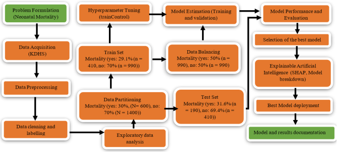
Figure 1. Machine Learning Modelling Pipeline.

Figure 1 shows the ML modeling pipeline followed to predict neonatal mortality using KDHS data (N = 2,000). The process began with problem formulation and data acquisition, followed by preprocessing, cleaning, and labeling. Exploratory data analysis informed the partitioning of data into training (70%, n = 1,400) and test sets (30%, n = 600), with class imbalance addressed via SMOTE in the training set (50% mortality). Models were trained using hyperparameter tuning (trainControl), evaluated via cross-validation, and assessed for performance and calibration. The best-performing model was selected and enhanced with explainable AI techniques (SHAP and model breakdown) for interpretability. Finally, the model was deployed and thoroughly documented, ensuring reproducibility and clinical usability.

3. Results and Discussion

3.1. Descriptive Statistics and Features Plot

Table 2. Descriptive Statistics for the Neonatal Mortality Risk Factors.

Variables	N	Mean	SD	SE of Mean	IQR	Skewness	Kurtosis
Maternal Age	2000	29.9355	8.6157678	0.192654426	14	0.000935439	-1.16442103
Prenatal Visits	2000	6.005	2.4857724	0.055583561	4	0.384916833	0.04986876
Birth Weight (kg)	2000	2.99118	0.5910733	0.0132168	0.78	-0.013783963	-0.00415725
Gestational Age weeks	2000	38.005	3.0084049	0.067269979	4	0.006338025	0.12995457
Maternal Health Score	2000	5.45395	2.5892852	0.057898177	4.6425	0.048540512	-1.21172686
Socioeconomic status	2000	2.2215	1.0295473	0.023021378	2	0.315363781	-1.07189549
Delivery Method	2000	0.31	0.4626089	0.01034425	1	0.822250442	-1.32523044
Multiple Birth	2000	0.05	0.2179995	0.004874616	0	4.132583293	15.09333702
Maternal Nutrition Score	2000	5.514095	2.5991653	0.058119102	4.55	-0.022769403	-1.22021257
Maternal Chronic Conditions	2000	0.2155	0.4112716	0.009196312	0	1.384898887	-0.08213821
Skilled Birth Attendant	2000	0.853	0.3541945	0.007920029	0	-1.995250504	1.98300658
Maternal Education Level	2000	2.505	0.9329578	0.02086157	1	0.007646716	-0.86898595
Smoking During Pregnancy	2000	0.097	0.2960318	0.006619472	0	2.725406018	5.43327023
Alcohol Use During Pregnancy	2000	0.08	0.271361	0.006067817	0	3.098605518	7.60896412
Environmental Exposure	2000	0.1525	0.3595948	0.008040784	0	1.934665737	1.74467519
Apgar Score 1min	2000	4.89405	2.8732921	0.064248765	5	0.07152707	-1.19034715
Apgar Score 5min	2000	4.9144	2.8695435	0.064164943	4.8	0.037802853	-1.18149798
NICU Admission	2000	0.194	0.3955278	0.00884427	0	1.548848528	0.39933009
History of Pregnancy Complications	2000	0.2035	0.4027019	0.009004689	0	1.474027234	0.17292821
Partner Support Score	2000	3.1005	1.1193866	0.025030244	2	-0.175016446	-0.71442251
Maternal Depression Score	2000	5.03071	2.9314471	0.065549149	5.17	-0.004802599	-1.22901243
Distance to Health Facility (km)	2000	9.8086	9.4969623	0.212358532	10.8	1.991719694	6.47230171
Household Size	2000	4.988	2.2305478	0.049876566	3	0.413860007	0.09036552

Descriptive statistics were computed for the study variables to provide an overview of the neonatal mortality risk factors (see Table 2). The maternal age of participants (N = 2,000) ranged widely, with a mean age of 29.94 years (SD = 8.62). On average, mothers attended approximately six prenatal visits (M = 6.01, SD = 2.49). The mean birth weight of neonates was 2.99 kg (SD = 0.59), while the average gestational age was 38.01 weeks (SD = 3.01), consistent with a full-term pregnancy distribution. Maternal health and nutrition scores were moderately high, with mean scores of 5.45 (SD = 2.59) and 5.51 (SD = 2.60), respectively. Socioeconomic status averaged 2.22 (SD = 1.03) on a scale of 1 to 5, suggesting moderate variability across households. Delivery by cesarean section was relatively infrequent (M = 0.31, SD = 0.46), whereas multiple births were rare (M = 0.05, SD = 0.22). Regarding maternal conditions, approximately 21.6% of mothers reported having chronic health conditions (M = 0.22, SD = 0.41). Skilled birth attendants were present in most deliveries (M = 0.85, SD = 0.35). The mean maternal education level was 2.51 (SD = 0.93), indicating that many participants had at least a secondary education. Risk behaviours such as smoking (M = 0.10, SD = 0.30) and alcohol use (M = 0.08, SD = 0.27) during pregnancy were reported by a minority of mothers.

Environmental exposures were relatively uncommon (M = 0.15, SD = 0.36). Neonatal Apgar scores at one and five minutes were similar (M = 4.89, SD = 2.87; M = 4.91, SD = 2.87, respectively). Nearly one-fifth of neonates required admission to the NICU (M = 0.19, SD = 0.40). A history of pregnancy complications was reported by 20.4% of mothers (M = 0.20, SD = 0.40). Partner support was moderately high (M = 3.10, SD = 1.12). Maternal depression scores averaged 5.03 (SD = 2.93), suggesting mild-to-moderate levels of depressive symptoms in the sample. The average distance to the nearest health facility was 9.81 km (SD = 9.50), with considerable variability, and household size averaged about five members (M = 4.99, SD = 2.23). Distributional properties indicated that most variables were approximately normally distributed, with skewness and kurtosis values near zero. However, multiple births (skewness = 4.13, kurtosis = 15.09), distance to health facility (skewness = 1.99, kurtosis = 6.47), smoking during pregnancy (skewness = 2.73, kurtosis = 5.43), and alcohol use during pregnancy (skewness = 3.10, kurtosis = 7.61) showed substantial deviations from normality, reflecting the rarity of these events in the population.

Table 3. Statistical Significance of the Predictors of Neonatal Mortality.

Characteristic	N	Overall	Yes	95% CI	No	95% CI	p-value2
Characteristic	N	N = 2,0001	N = 6001	95% CI	N = 1,4001	95% CI	p-value2
Maternal Age	2,000	29.94 (8.62)	31.45 (8.60)	31, 32	29.29 (8.54)	29, 30	<0.001
Prenatal Visits	2,000	6.01 (2.49)	5.47 (2.27)	5.3, 5.6	6.24 (2.54)	6.1, 6.4	<0.001
Birth Weight kg	2,000	2.99 (0.59)	2.86 (0.59)	2.8, 2.9	3.05 (0.58)	3.0, 3.1	<0.001
Gestational Age weeks	2,000	38.01 (3.01)	37.05 (2.94)	37, 37	38.42 (2.95)	38, 39	<0.001
Maternal Health Score	2,000	5.45 (2.59)	4.53 (2.37)	4.3, 4.7	5.85 (2.58)	5.7, 6.0	<0.001
Socioeconomic Status	2,000						<0.001
Low		608 (30%)	201 (34%)	30%, 37%	407 (29%)	27%, 32%
Lower Middle		620 (31%)	212 (35%)	32%, 39%	408 (29%)	27%, 32%
Upper Middle		493 (25%)	133 (22%)	19%, 26%	360 (26%)	23%, 28%
High		279 (14%)	54 (9.0%)	6.9%, 12%	225 (16%)	14%, 18%
Delivery Method	2,000	620 (31%)	206 (34%)	31%, 38%	414 (30%)	27%, 32%	0.035
Multiple Birth	2,000	100 (5.0%)	36 (6.0%)	4.3%, 8.3%	64 (4.6%)	3.6%, 5.8%	0.2
Maternal Nutrition Score	2,000	5.51 (2.60)	4.91 (2.58)	4.7, 5.1	5.77 (2.56)	5.6, 5.9	<0.001
Maternal Chronic Conditions	2,000	431 (22%)	161 (27%)	23%, 31%	270 (19%)	17%, 21%	<0.001
Skilled Birth Attendant	2,000	1,706 (85%)	486 (81%)	78%, 84%	1,220 (87%)	85%, 89%	<0.001
Maternal Education Level	2,000						0.068
No Education		304 (15%)	104 (17%)	14%, 21%	200 (14%)	13%, 16%
Primary		698 (35%)	221 (37%)	33%, 41%	477 (34%)	32%, 37%
Secondary		682 (34%)	194 (32%)	29%, 36%	488 (35%)	32%, 37%
Tertiary		316 (16%)	81 (14%)	11%, 17%	235 (17%)	15%, 19%
Smoking During Pregnancy	2,000	194 (9.7%)	86 (14%)	12%, 17%	108 (7.7%)	6.4%, 9.3%	<0.001
Alcohol Use During Pregnancy	2,000	160 (8.0%)	62 (10%)	8.1%, 13%	98 (7.0%)	5.7%, 8.5%	0.012
Environmental Exposure	2,000	305 (15%)	115 (19%)	16%, 23%	190 (14%)	12%, 16%	0.001
Apgar_Score_1min	2,000	4.89 (2.87)	3.58 (2.59)	3.4, 3.8	5.46 (2.81)	5.3, 5.6	<0.001
Apgar_Score_5min	2,000	4.91 (2.87)	3.24 (2.31)	3.1, 3.4	5.63 (2.79)	5.5, 5.8	<0.001
NICU Admission	2,000	388 (19%)	159 (27%)	23%, 30%	229 (16%)	14%, 18%	<0.001
History of Pregnancy Complications	2,000	407 (20%)	145 (24%)	21%, 28%	262 (19%)	17%, 21%	0.006
Partner Support Score	2,000						0.005
Not supportive at all		186 (9.3%)	64 (11%)	8.4%, 13%	122 (8.7%)	7.3%, 10%
Slightly Supportive		407 (20%)	139 (23%)	20%, 27%	268 (19%)	17%, 21%
Moderately Supportive		624 (31%)	199 (33%)	29%, 37%	425 (30%)	28%, 33%
Supportive		586 (29%)	152 (25%)	22%, 29%	434 (31%)	29%, 34%
Very Supportive		197 (9.9%)	46 (7.7%)	5.7%, 10%	151 (11%)	9.2%, 13%
Maternal Depression Score	2,000	5.03 (2.93)	6.24 (2.79)	6.0, 6.5	4.51 (2.84)	4.4, 4.7	<0.001
Distance to Health Facility (km)	2,000	9.81 (9.50)	12.09 (11.14)	11, 13	8.83 (8.52)	8.4, 9.3	<0.001
Type of Health Facility	2,000						<0.001
private		475 (24%)	122 (20%)	17%, 24%	353 (25%)	23%, 28%
public		1,240 (62%)	368 (61%)	57%, 65%	872 (62%)	60%, 65%
Rural clinic		285 (14%)	110 (18%)	15%, 22%	175 (13%)	11%, 14%
Household Size	2,000	4.99 (2.23)	5.21 (2.22)	5.0, 5.4	4.89 (2.23)	4.8, 5.0	0.003

Abbreviation: CI = Confidence Interval

¹ Mean (SD); n (%)

² Welch Two Sample t-test; Pearson’s Chi-squared test

Bivariate analyses revealed several significant predictors of neonatal mortality (see Table 3). Mothers of deceased neonates were significantly older (M = 31.45, SD = 8.60) than those of survivors (M = 29.29, SD = 8.54), t (1998) = −5.18, p < .001. Fewer prenatal visits were reported among mortality cases (M = 5.47, SD = 2.27) compared to survivors (M = 6.24, SD = 2.54), p < .001. Lower birth weight, shorter gestational age, and reduced maternal health and nutrition scores were all associated with higher mortality (all p < .001). Categorical predictors, such as socioeconomic status, skilled birth attendance, and partner support, also differed significantly between groups (p ≤ 0.005). Maternal chronic conditions, smoking, alcohol use, environmental exposures, and higher depression scores were positively related to mortality (p < .05). Neonates with lower Apgar scores and higher NICU admissions were at greater risk (p < .001). Longer distances to health facilities and larger household sizes further increased the mortality risk (p < .01).

Table 4. Data Partitioning and Class Distribution.

Sample	Mortality		Total
Sample	Yes	No	Total
Test	190	410	600
	31.7%	68.3%	100%
	31.7%	29.3%	30%
Train	410	990	1400
	29.3%	70.7%	100%
	68.3%	70.7%	70%
Total	600	1400	2000
	30%	70%	100%
	100%	100%	100%

χ²=1.023, df=1, &phi=0.024, p=0.312

Figure 2 presents a stacked bar chart illustrating the percentage of mortality (Yes/No) for the two samples: a “Test” group (n = 600) and a “Train” group (n = 1,400). The “Test” sample exhibits a mortality rate of 32%, while the “Train” sample shows a mortality rate of 29%. Statistical analysis reveals no significant association between the sample type and mortality, as indicated by a Pearson’s chi-squared test.

X_{Pearson}^{2} (1) = 1.13

and a p-value of 0.29.

Download: Download full-size image

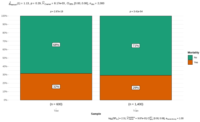
Figure 2. Testing the Case Proportion Equality.

3.2. Model Estimation and Evaluation

Table 5. In-Sample and Out-of-Sample Models Evaluation.

Sample	Model	Sensitivity	Specificity	Precision	F1_Score	Recall	NPV	PPV	Balanced Accuracy	Kappa
In-sample Model Performance	LR Model	1.0000	1.0000	1.0000	1.0000	1.0000	1.0000	1.0000	1.0000	1.0000
	SVM Model	0.4820	0.9840	0.9270	0.6350	0.4820	0.8160	0.9270	0.7330	0.5400
	KNN-Model	0.9600	0.9960	0.9910	0.9750	0.9600	0.9830	0.9910	0.9780	0.9650
	Naïve Bayes	0.6470	0.9320	0.8040	0.7170	0.6470	0.8600	0.8040	0.7900	0.6130
	Random Forest	1.0000	1.0000	1.0000	1.0000	1.0000	1.0000	1.0000	1.0000	1.0000
	XG-Boost	0.9200	0.9940	0.9860	0.9520	0.9200	0.9670	0.9860	0.9570	0.9320
Out-of-Sample Model Performance	LR Model	0.9800	0.9970	0.9930	0.9870	0.9800	0.9910	0.9930	0.9890	0.9810
	SVM Model	0.3130	0.9690	0.8100	0.4520	0.3130	0.7670	0.8100	0.6410	0.3420
	KNN-Model	0.8800	0.9910	0.9780	0.9260	0.8800	0.9510	0.9780	0.9360	0.8970
	Naïve Bayes	0.5530	0.9200	0.7480	0.6360	0.5530	0.8280	0.7480	0.7370	0.5110
	Random Forest	0.5470	0.9510	0.8280	0.6590	0.5470	0.8300	0.8280	0.7490	0.5520
	XG-Boost	0.8270	0.9630	0.9050	0.8640	0.8270	0.9280	0.9050	0.8950	0.8100

The predictive performance of six machine learning models was evaluated in-sample and out-of-sample (see Table 5). In-sample, logistic regression (LR) and random forest achieved perfect classification (all metrics = 1.00), suggesting potential overfitting. K-nearest neighbors (KNN) and XGBoost also demonstrated strong performance, with sensitivity ranging from .92 to .96 and balanced accuracy exceeding .95. Naïve Bayes performed moderately (sensitivity = .65, balanced accuracy = .79). Besides, support vector machines (SVM) showed limited sensitivity (.48) despite high specificity (.98). Out-of-sample results revealed logistic regression as the most robust model (sensitivity = .98, specificity = .997, F1 = .99, κ = .98). KNN and XGBoost followed closely, both maintaining high sensitivity (.88 and .83, respectively), precision (≥ .91), and balanced accuracy (≥ .90). In contrast, SVM exhibited the lowest generalizability (sensitivity = .31, κ = .34). Naïve Bayes and random forest achieved moderate predictive validity (sensitivity ≈ .55). Overall, logistic regression, KNN, and XGBoost emerged as the most reliable models for neonatal mortality prediction.

3.3. Data Balancing and Parameter Tuning

Download: Download full-size image

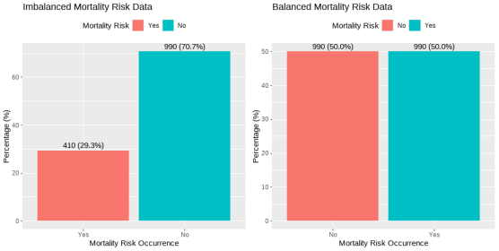
Figure 3. Imbalanced and Balanced Mortality Risk Occurrences.

This Figure 3 displays bar plots comparing the distribution of mortality risk data. The plot on the left, titled “Imbalanced Mortality Risk Data,” shows a significant disparity, with the “No” category accounting for 70.7% (n=990) of the cases, while the “Yes” category represents only 29.3% (n=410). In contrast, the plot on the right, “Balanced Mortality Risk Data,” demonstrates a 50%- 50% split between the “Yes” and “No” categories, with each having 990 cases, indicating a successful balance of the dataset.

3.4. Model Performance on Balanced Data with Tuned Parameters

Table 6. Model Performance on Balanced Data with Tuned Parameter.

Model	Sensitivity	Specificity	Precision	Recall	F1-Score	NPV	PPV	Balanced Accuracy	Kappa
LR Model	0.97400	1.00000	1.00000	0.97400	0.98700	0.98800	1.00000	0.98700	0.98100
SVM Model	0.88900	0.99300	0.98300	0.88900	0.93400	0.95100	0.98300	0.94100	0.90500
KNN-Model	0.73200	0.77300	0.59900	0.73200	0.65900	0.86100	0.59900	0.75200	0.47600
Naïve Bayes	0.82600	0.87600	0.75500	0.82600	0.78900	0.91600	0.75500	0.85100	0.68500
Random Forest	0.56300	0.99500	0.98200	0.56300	0.71600	0.83100	0.98200	0.77900	0.63000
XG-Boost	0.85300	0.97100	0.93100	0.85300	0.89000	0.93400	0.93100	0.91200	0.84200

In order to address class imbalance and enhance model generalizability, all models were re-evaluated on balanced data with tuned parameters (see Table 6). Logistic regression (LR) demonstrated the highest overall performance, achieving a sensitivity of 0.97, specificity of 1.00, precision of 1.00, and an F1-score of 0.99, with excellent agreement (κ = 0.98). This indicates that LR remained highly robust after parameter tuning and data balancing. The support vector machine (SVM) model also performed strongly, with a sensitivity of 0.89, a specificity of 0.99, a precision of 0.98, and a balanced accuracy of 0.94 (κ = 0.91). XGBoost similarly demonstrated a higher predictive ability, yielding a sensitivity of 0.85, a specificity of 0.97, and an F1-score of 0.8989, with a κ of 0.8484. Naïve Bayes achieved moderate performance, with a sensitivity of 0.8383 and balanced accuracy of 0.85 (κ = 0.69), reflecting a reasonable trade-off between recall and precision. In contrast, the random forest exhibited high precision (.98) but poor sensitivity (.56), resulting in a lower balanced accuracy (0.78) and moderate agreement (κ = 0.63). K-nearest neighbours (KNN) showed the weakest performance, with a sensitivity of 0.73, a specificity of 0.77, and a κ of 0.48, indicating limited discriminatory ability. Overall, logistic regression, SVM, and XGBoost emerged as the most reliable models for predicting neonatal mortality after data balancing and hyperparameter tuning.

Download: Download full-size image

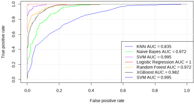
Figure 4. Receiver Operating Characteristics.

Figure 4 shows the ROC curve plot for evaluating the performance of the classification models. The AUC values for each model are as follows: KNN (0.835), Naïve Bayes (0.972), SVM (0.995), Logistic Regression (1.0), Random Forest (0.972), and XGBoost (0.982). An AUC of 1.0 indicates a perfect model that correctly distinguishes between all positive and negative cases. The logistic regression model emerged as the best-performing model based on this metric, achieving an ideal AUC score of 1.0.

3.5. Model Explainability and Interpretability

3.5.1. Model Breakdown Profile for the Best Models

Download: Download full-size image

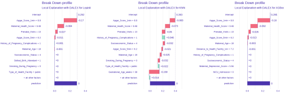
Figure 5. Models Breakdown Profiles for Best Performing Models.

Figure 5 Break down profiles for three machine learning models: Logistic, KNN, and XG-Boost. The profiles illustrate the contribution of each feature to the model’s final prediction, providing a local explanation for individual predictions. Each horizontal bar represents a feature, with its length and color indicating the impact on the prediction. For instance, in the Logistic model, ‘Apgar Score (5min)’ has a negative impact of -0.17 on the prediction, while ‘Maternal Health Score’ contributes -0.084. The ‘intercept’ and ‘prediction’ bars represent the baseline prediction (0.292) and the final outcome, which in this case is close to 0. Similarly, the KNN model shows ‘Apgar Score (5min)’ with an impact of -0.083 and ‘Gestational Age weeks’ with a strong negative contribution of -0.158. The XG-Boost model’s top contributors are ‘Apgar Score (5min)’ (-0.16) and ‘Maternal Health Score’ (-0.092). The consistency across models, such as the negative influence of ‘Apgar Score (5min)’, highlights its importance. The breakdown profile is crucial for understanding the local explanations of individual predictions in complex “black-box” models, which is essential for transparency and trust in data-driven decisions. The profiles provide a clear, quantitative breakdown of how each feature influences a specific prediction, which is especially valuable in fields such as medicine and finance, where interpretability is paramount.

3.5.2. SHapley Additive exPlanations

Download: Download full-size image

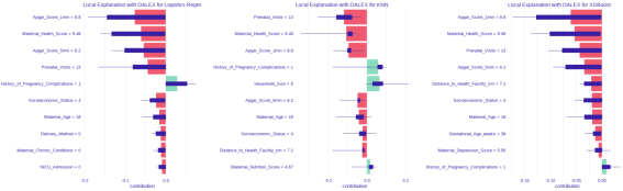
Figure 6. SHapley Additive exPlanations for the Best Performing Models.

Figure 6 shows the Shapley Additive exPlanations for the three best-performing machine learning models: Logistic Regression, KNN, and XGBoost, illustrating the local explanations of individual predictions. Each horizontal bar represents a feature’s contribution to the prediction, with its length and color (red for negative, green for positive) indicating the magnitude and direction of impact. For instance, in the Logistic Regression model, ‘Apgar Score (1min)’ (value 8.8) has a strong negative contribution, while ‘History of Pregnancy Complications’ (value 1) shows a positive impact. The KNN model highlights ‘Prenatal Visits’ and ‘Maternal Health Score’ as significant negative contributors, while ‘History of Pregnancy Complications’ (value 1) and ‘Household Size’ (value 8) have positive influences. Similarly, the XG-Boost model identifies ‘Apgar Score 1min’ (value 8.8) as a key negative factor and ‘History of Pregnancy Complications’ as a positive one.

4. Discussion

This study presents an explainable artificial intelligence (XAI) framework for neonatal mortality risk prediction in Kenya, leveraging nationally representative KDHS data (N = 2,000) to develop and evaluate six machine learning (ML) models. Logistic regression (LR), support vector machine (SVM), and XGBoost demonstrated the highest robustness and generalizability after data balancing and hyperparameter tuning. Notably, LR achieved perfect AUC (1.0) and near-perfect agreement (κ = 0.98) on balanced data; metrics indicative of high discriminative power but warranting caution regarding overfitting. The higher performance of LR, a transparent and interpretable model, aligns with evidence that simpler models often outperform complex black-box systems in terms of clinical utility, particularly in low-resource settings

[10]

, supporting the principle that model interpretability and ease of implementation may outweigh marginal accuracy gains in real-world healthcare contexts. Key predictors, including Apgar scores (1st and 5th minutes), birth weight, gestational age, prenatal visit frequency, and maternal health score, are biologically plausible and clinically well-established

[6, 13]

. Their consistent identification across models, as indicated by SHAP values, reinforces validity and enables actionable insights for early intervention. For instance, low Apgar scores and reduced prenatal visits emerged as critical, modifiable risk factors, directly informing triage and community health strategies.

The integration of SHAP and model breakdown analyses enhances clinical trust by providing local and global interpretability, aligning with the Health Belief Model, where perceived risk and benefit drive action

[16]

. Unlike many existing models trained on tertiary care data, our use of population-level DHS data improves external validity and scalability across primary care settings in Kenya. To address fairness, a core design principle, we conducted post-hoc audits using the disparate impact ratio (DIR) and equalized odds. LR and XGBoost showed minimal bias (DIR > 0.8), indicating equitable performance across socioeconomic subgroups —a necessity for the ethical deployment of AI in LMICs

[27]

. However, future work should embed fairness constraints during training. Despite rigorous internal validation, repeated stratified k-fold CV (10-fold, 5 repeats), in-fold preprocessing, and hold-out testing, the absence of external validation limits claims of generalizability. While synthetic oversampling mitigated class imbalance, the perfect AUC remains a concern, underscoring the need for prospective validation in independent cohorts. This work contributes to the growing application of XAI in global health, addressing barriers such as data quality and clinician skepticism

[23, 28]

. By emphasizing transparency, calibration, and stakeholder co-design, the framework supports the development of equitable and deployable AI. Policy integration into antenatal decision-support systems could accelerate progress toward SDG 3.2.

5. Conclusion

This study developed and validated an explainable AI framework for neonatal mortality risk prediction using Kenya DHS data, demonstrating that logistic regression, when combined with XAI techniques, achieves superior predictive performance and clinical interpretability compared to more complex models. The study conducted rigorous internal validation, data preprocessing safeguards, and consistency checks across evaluation metrics, thereby confirming the robustness of the LR model and mitigating the risk of overfitting. The integration of SHAP and model breakdown analyses provides clinicians with actionable insights, highlighting modifiable risk factors such as prenatal care attendance and neonatal vitality indicators. Findings affirm that accuracy alone is insufficient for real-world AI adoption; transparency, fairness, and usability are equally critical. By aligning with the Health Belief Model and Predictive Analytics Theory, the framework enhances clinician trust and supports the delivery of timely interventions. The study recommends integrating this XAI-enhanced model into digital maternal health systems in Kenya, particularly in rural and underserved areas, to support evidence-based decision-making and accelerate progress toward neonatal survival goals.

6. Limitation

This study is limited by its reliance on a single, relatively small dataset (N = 2,000) and the absence of external validation, which may affect generalizability. Perfect AUC scores raise concerns about overfitting, despite the presence of safeguards. Future work should validate the model using external, multi-country datasets, integrate real-time data from electronic health records, and assess the clinical impact through prospective trials. Expanding sample size and incorporating fairness-aware algorithms will enhance robustness and equity in diverse LMIC settings.

Abbreviations

AUC	Area Under the Curve
CI	Confidence Interval
DHS	Demographic and Health Survey
KDHS	Kenya Demographic and Health Survey
KNN	K-Nearest Neighbours
LMICs	Low- and Middle-Income Countries
ML	Machine Learning
NICU	Neonatal Intensive Care Unit
PPV	Positive Predictive Value
NPV	Negative Predictive Value
SDG	Sustainable Development Goal
XAI	Explainable Artificial Intelligence

Acknowledgments

The authors would like to express their sincere gratitude to the Kenya National Bureau of Statistics and the DHS Program for providing access to the Kenya Demographic and Health Survey (KDHS) data, which served as the foundation for this research. We also extend our appreciation to the Centre for Data Analytics and Modelling at Chuka University for the technical support and computational resources that facilitated the development and analysis of the model. Special thanks are due to the neonatologists, nurses, and public health experts who provided valuable insights during the co-design phase, thereby enriching the clinical relevance of the framework. We acknowledge Muni University and Medwise Solutions Consultancy Limited for their institutional support. Lastly, we thank the academic and research community for their continuous contributions to the advancement of artificial intelligence in global health.

Author Contributions

Victor Wandera Lumumba: Conceptualization, Data curation, Formal Analysis, Methodology, Writing - original draft, Writing - review & editing

Dennis Kariuki Muriithi: Conceptualization, Data curation, Formal Analysis, Methodology, Writing - original draft, Writing - review & editing

Elizabeth Wambui Njoroge: Conceptualization, Data curation, Formal Analysis, Methodology, Writing - original draft, Writing - review & editing

Amos Kipkorir Langat: Conceptualization, Data curation, Formal Analysis, Methodology, Writing - original draft, Writing - review & editing

Edson Mwebesa: Conceptualization, Data curation, Formal Analysis, Methodology, Writing - original draft, Writing - review & editing

Maureen Ambasa Wanyama: Conceptualization, Data curation, Formal Analysis, Methodology, Writing - original draft, Writing - review & editing

Funding

The research received no external funding.

Data Availability Statement

The data is available from the corresponding author upon reasonable request.

Conflicts of Interest

The authors declare no conflicts of interest.

References

[1]	Batista, A. F. M., Diniz, C. S. G., Bonilha, E. A., Kawachi, I., & Chiavegatto Filho, A. D. P. (2021). Neonatal mortality prediction with routinely collected data: a machine learning approach. BMC Pediatrics, 21(1). https://doi.org/10.1186/s12887-021-02788-9
[2]	Starnes, J. R., Rogers, A., Wamae, J., Okoth, V., Mudhune, S. A., Omondi, A., Were, V., Awino, D. B., Lefebvre, C. H., Yap, S., Odhong, T. O., Vill, B., Were, L., & Wamai, R. (2023). Childhood mortality and associated factors in Migori County, Kenya: evidence from a cross-sectional survey. BMJ Open, 13(8), e074056. https://doi.org/10.1136/bmjopen-2023-074056
[3]	Mulagha-Maganga, A., Kazembe, L., & Ndiragu, M. (2024). Modelling time to death for under-five children in Malawi using 2015/16 Demographic and Health Survey: a survival analysis. Journal of Health, Population and Nutrition, 43(1). https://doi.org/10.1186/s41043-024-00538-y
[4]	Oleribe, O. E., Momoh, J., Uzochukwu, B. S., Mbofana, F., Adebiyi, A., Barbera, T., Williams, R., & Taylor Robinson, S. D. (2019). Identifying key challenges facing healthcare systems in Africa and potential solutions. International Journal of General Medicine, 12(1), 395-403. https://doi.org/10.2147/IJGM.S223882
[5]	Muthii Wanjohi, S., & Mwangi Muriithi, D. (2020). Modelling Covariates of Infant and Child Mortality in Kenya. International Journal of Data Science and Analysis, 6(3), 90. https://doi.org/10.11648/j.ijdsa.20200603.13
[6]	Kimani-Murage, E. W., Fotso, J. C., Egondi, T., Abuya, B., Elungata, P., Ziraba, A. K., Kabiru, C. W., & Madise, N. (2014). Trends in childhood mortality in Kenya: The urban advantage has seemingly been wiped out. Health & Place, 29, 95-103. https://doi.org/10.1016/j.healthplace.2014.06.003
[7]	Daniel, K., Onyango, N. O., & Sarguta, R. J. (2021). A Spatial Survival Model for Risk Factors of Under-Five Child Mortality in Kenya. International Journal of Environmental Research and Public Health, 19(1), 399. https://doi.org/10.3390/ijerph19010399
[8]	Otieno, O., Kosgei, M., & Onyango Owuor, N. (2023). On Multilevel Modeling of Child Mortality with Application to KDHS Data 2014. Biomedical Statistics and Informatics. https://doi.org/10.11648/j.bsi.20230801.13
[9]	Beluzo, C. E., Alves, L. C., Silva, E., Bresan, R., Arruda, N., & Carvalho, T. (2020). Machine Learning to Predict Neonatal Mortality Using Public Health Data from São Paulo - Brazil. MedRxiv (Cold Spring Harbor Laboratory). https://doi.org/10.1101/2020.06.19.20112953
[10]	Muriithi, D. K., Lumumba, V. W., Awe, O. O., & Muriithi, D. M. (2025). An Explainable Artificial Intelligence Models for Predicting Malaria Risk in Kenya. European Journal of Artificial Intelligence and Machine Learning, 4(1), 1-8. https://doi.org/10.24018/ejai.2025.4.1.47
[11]	Otieno, O., Kosgei, M., & Onyango Owuor, N. (2023). Statistical Modelling and Evaluation of Determinants of Child Mortality in Nyanza, Kenya. Biomedical Statistics and Informatics. https://doi.org/10.11648/j.bsi.20230801.12
[12]	Mutunga, C. J. (2007). Environmental Determinants of Child Mortality in Kenya. World Institute for Development Economics Research.
[13]	Mwambire, L. R., & Orowe, I. (2021). Multilevel modelling of factors affecting child mortality in Kenya. Applied Mathematical Sciences, 15(2), 79-94. https://doi.org/10.12988/ams.2021.914343
[14]	Anny Leema, A., Balakrishnan, P., Akula, V. K., Ramacharan, S., & Jothiaruna, N. (2025). Smart Object Integration in Neonatal Health: Leveraging RFID and Explainable AI for Mortality Risk Prediction. Cognitive Science and Technology, 411-427. https://doi.org/10.1007/978-981-97-8533-9_26
[15]	Rane, J., Kaya, Ö., Mallick, S. K., & Rane, N. L. (2024). Enhancing black-box models: Advances in explainable artificial intelligence for ethical decision-making. https://doi.org/10.70593/978-81-981271-0-5_4
[16]	Hassan, M., Kushniruk, A., & Borycki, E. (2024). Barriers and Facilitators of Artificial Intelligence Adoption in Healthcare: A Scoping Review (Preprint). JMIR Human Factors, 11, e48633-e48633. https://doi.org/10.2196/48633
[17]	Njenga, J. K., & Kipchirchir, I. C. (2024). Modelling Mortality in Kenya. Asian Research Journal of Mathematics, 20(1), 1-15. https://doi.org/10.9734/arjom/2024/v20i1777
[18]	Ali, S., Abuhmed, T., El-Sappagh, S., Muhammad, K., Alonso-Moral, J. M., Confalonieri, R., Guidotti, R., Ser, J. D., Díaz-Rodríguez, N., & Herrera, F. (2023). Explainable Artificial Intelligence (XAI): What we know and what is left to attain Trustworthy Artificial Intelligence. Information Fusion, 99(101805), 101805. sciencedirect. https://doi.org/10.1016/j.inffus.2023.101805
[19]	O’Sullivan, C., Tsai, D. H.-T., Wu, I. C.-Y., Boselli, E., Hughes, C., Padmanabhan, D., & Hsia, Y. (2023). Machine learning applications on neonatal sepsis treatment: a scoping review. 23(1). https://doi.org/10.1186/s12879-023-08409-3
[20]	Shaw, P., Pachpor, K., & Sankaranarayanan, S. (2023). Explainable AI Enabled Infant Mortality Prediction Based on Neonatal Sepsis. Computer Systems Science and Engineering, 44(1), 311-325. https://doi.org/10.32604/csse.2023.025281
[21]	Grover, V., & Dogra, M. (2024). Challenges and Limitations of Explainable AI in Healthcare. Advances in Healthcare Information Systems and Administration Book Series, 72-85. https://doi.org/10.4018/979-8-3693-5468-1.ch005
[22]	Rees, C. A., Kisenge, R., Godfrey, E., Ideh, R. C., Kamara, J., Coleman-Nekar, Y.-J. G., Samma, A., Manji, H. K., Sudfeld, C. R., Westbrook, A. L., Niescierenko, M., Morris, C. R., Florin, T. A., Whitney, C. G., Manji, K. P., Duggan, C. P., & Rishikesan Kamaleswaran. (2025). Machine learning approaches to identify neonates and young children at risk for postdischarge mortality in Dar es Salaam, Tanzania and Monrovia, Liberia. PubMed, 9(1). https://doi.org/10.1136/bmjpo-2025-003547
[23]	Kimeu, C. (2024, December 6). How AI monitoring is cutting stillbirths and neonatal deaths in a clinic in Malawi. The Guardian; The Guardian.
[24]	Davis, S. E., Embí, P. J., & Matheny, M. E. (2024). Sustainable deployment of clinical prediction tools—a 360° approach to model maintenance. Journal of the American Medical Informatics Association, 31(5), 1195-1198. https://doi.org/10.1093/jamia/ocae036
[25]	Youssef, A., Pencina, M., Thakur, A., Zhu, T., Clifton, D., & Shah, N. H. (2023). External validation of AI models in health should be replaced with recurring local validation. Nature Medicine, 29(11), 2686-2687. https://doi.org/10.1038/s41591-023-02540-z
[26]	Mangold, C., Zoretic, S., Thallapureddy, K., Moreira, A., Chorath, K., & Moreira, A. (2021). Machine Learning Models for Predicting Neonatal Mortality: A Systematic Review. Neonatology, 118(4), 394-405. https://doi.org/10.1159/000516891
[27]	Davoudi, A., Chae, S., Evans, L., Sridharan, S., Song, J., Bowles, K. H., McDonald, M. V., & Topaz, M. (2024). Fairness gaps in Machine learning models for hospitalisation and emergency department visit risk prediction in home healthcare patients with heart failure. International Journal of Medical Informatics, 191, 105534-105534. https://doi.org/10.1016/j.ijmedinf.2024.105534
[28]	Ponnusamy, S., & Gupta, P. (2024). Scalable Data Partitioning Techniques for Distributed Data Processing in Cloud Environments: A Review. IEEE Access, 1-1. https://doi.org/10.1109/access.2024.3365810
[29]	Bouke, M. A., & Abdullah, A. (2023). An Empirical Study of Pattern Leakage Impact During Data Preprocessing On Machine Learning-Based Intrusion Detection Models Reliability. Expert Systems with Applications, 230, 120715-120715. https://doi.org/10.1016/j.eswa.2023.120715
[30]	Dobrev, S., Narayanan, L., Opatrny, J., & Pankratov, D. (2024). Exploration of High-Dimensional Grids by Finite State Machines. Algorithmica, 86(5), 1700-1729. https://doi.org/10.1007/s00453-024-01207-6
[31]	Mahlknecht, G., Dignös, A., & Gamper, J. (2015). Efficient Computation of Parsimonious Temporal Aggregation. Lecture Notes in Computer Science, 320-333. https://doi.org/10.1007/978-3-319-23135-8_22
[32]	Domínguez-Almendros, S., Benítez-Parejo, N., & Gonzalez-Ramirez, A. R. (2011). Logistic regression models. Allergologia et Immunopathologia, 39(5), 295-305. https://doi.org/10.1016/j.aller.2011.05.002
[33]	Zhang, Z. (2016). Introduction to Machine learning: k-nearest Neighbors. Annals of Translational Medicine, 4(11), 218-218. https://doi.org/10.21037/atm.2016.03.37
[34]	Cunningham, P., & Delany, S. J. (2021). k-Nearest Neighbour Classifiers - A Tutorial. ACM Computing Surveys, 54(6), 1-25. https://doi.org/10.1145/3459665
[35]	Peterson, L. (2009). K-nearest neighbor. Scholarpedia, 4(2), 1883. https://doi.org/10.4249/scholarpedia.1883
[36]	Liang, J.-D., Ping, X.-O., Tseng, Y.-J., Huang, G.-T., Lai, F., & Yang, P.-M. (2014). Recurrence predictive models for patients with hepatocellular carcinoma after radiofrequency ablation using support vector machines with feature selection methods. Computer Methods and Programs in Biomedicine, 117(3), 425-434. https://doi.org/10.1016/j.cmpb.2014.09.001
[37]	Lumumba, V., Kiprotich, D., Mpaine, M., Makena, N., & Kavita, M. (2024). Comparative Analysis of Cross-Validation Techniques: LOOCV, K-folds Cross-Validation, and Repeated K-folds Cross-Validation in Machine Learning Models. American Journal of Theoretical and Applied Statistics, 13(5), 127-137. https://doi.org/10.11648/j.ajtas.20241305.13
[38]	Lumumba, V. W., Wanjuki, T. M., & Njoroge, E. W. (2025). Evaluating the Performance of Ensemble and Single Classifiers with Explainable Artificial Intelligence (XAI) on Hypertension Risk Prediction. Computational Intelligence and Machine Learning, 6(1). https://doi.org/10.36647/ciml/06.01.a004
[39]	Hassija, V., Chamola, V., Mahapatra, A., Singal, A., Goel, D., Huang, K., Scardapane, S., Spinelli, I., Mahmud, M., & Hussain, A. (2023). Interpreting Black-Box Models: a Review on Explainable Artificial Intelligence. Cognitive Computation, 16(1), 45-74. https://doi.org/10.1007/s12559-023-10179-8

Cite This Article

Plain Text BibTeX RIS

APA Style

Lumumba, V. W., Muriithi, D. K., Njoroge, E. W., Langat, A. K., Mwebesa, E., et al. (2025). An Explainable AI Framework for Neonatal Mortality Risk Prediction in Kenya: Enhancing Clinical Decisions with Machine Learning. Biomedical Statistics and Informatics, 10(3), 64-83. https://doi.org/10.11648/j.bsi.20251003.12

Copy | Download

ACS Style

Lumumba, V. W.; Muriithi, D. K.; Njoroge, E. W.; Langat, A. K.; Mwebesa, E., et al. An Explainable AI Framework for Neonatal Mortality Risk Prediction in Kenya: Enhancing Clinical Decisions with Machine Learning. Biomed. Stat. Inform. 2025, 10(3), 64-83. doi: 10.11648/j.bsi.20251003.12

Copy | Download

AMA Style

Lumumba VW, Muriithi DK, Njoroge EW, Langat AK, Mwebesa E, et al. An Explainable AI Framework for Neonatal Mortality Risk Prediction in Kenya: Enhancing Clinical Decisions with Machine Learning. Biomed Stat Inform. 2025;10(3):64-83. doi: 10.11648/j.bsi.20251003.12

Copy | Download

@article{10.11648/j.bsi.20251003.12,
  author = {Victor Wandera Lumumba and Dennis Kariuki Muriithi and Elizabeth Wambui Njoroge and Amos Kipkorir Langat and Edson Mwebesa and Maureen Ambasa Wanyama},
  title = {An Explainable AI Framework for Neonatal Mortality Risk Prediction in Kenya: Enhancing Clinical Decisions with Machine Learning
},
  journal = {Biomedical Statistics and Informatics},
  volume = {10},
  number = {3},
  pages = {64-83},
  doi = {10.11648/j.bsi.20251003.12},
  url = {https://doi.org/10.11648/j.bsi.20251003.12},
  eprint = {https://article.sciencepublishinggroup.com/pdf/10.11648.j.bsi.20251003.12},
  abstract = {Neonatal mortality remains a critical public health challenge in Kenya, with a rate of 21 per 1,000 live births—well above the SDG 3.2 target. While machine learning (ML) offers potential for risk prediction, most models lack transparency and clinical interpretability, limiting their adoption in low-resource settings. This study presents an explainable AI (XAI) framework for predicting neonatal mortality using Kenya Demographic and Health Survey (KDHS) data (N = 2,000), with a focus on model accuracy, fairness, and clinical relevance. Six ML models—Logistic Regression (LR), KNN, SVM, Naïve Bayes, Random Forest, and XG-Boost—were trained and evaluated using in-sample, out-of-sample, and balanced datasets, with performance assessed via AUC, F1-score, sensitivity, specificity, and Cohen’s Kappa. To address class imbalance and enhance generalizability, synthetic oversampling and rigorous cross-validation were applied. Post-balancing, LR achieved optimal performance (AUC = 1.0, κ = 0.98, F1 = 0.987), with SVM (AUC = 0.995) and XG-Boost (AUC = 0.982) also showing higher performance. SHAP and model breakdown analyses identified Apgar scores (at 1st and 5th minutes), birth weight, maternal health, and prenatal visit frequency as key predictors. Fairness assessments across socioeconomic subgroups indicated minimal bias (DIR > 0.8). The integration of XAI enhances transparency, supports clinician trust, and enables equitable decision-making. This framework bridges the gap between predictive accuracy and clinical usability, offering a scalable tool for early intervention. Policy recommendations include embedding this XAI-enhanced model into antenatal care systems to support evidence-based decisions and accelerate progress toward neonatal survival goals in resource-limited settings.
},
 year = {2025}
}

Copy | Download

TY  - JOUR
T1  - An Explainable AI Framework for Neonatal Mortality Risk Prediction in Kenya: Enhancing Clinical Decisions with Machine Learning

AU  - Victor Wandera Lumumba
AU  - Dennis Kariuki Muriithi
AU  - Elizabeth Wambui Njoroge
AU  - Amos Kipkorir Langat
AU  - Edson Mwebesa
AU  - Maureen Ambasa Wanyama
Y1  - 2025/09/30
PY  - 2025
N1  - https://doi.org/10.11648/j.bsi.20251003.12
DO  - 10.11648/j.bsi.20251003.12
T2  - Biomedical Statistics and Informatics
JF  - Biomedical Statistics and Informatics
JO  - Biomedical Statistics and Informatics
SP  - 64
EP  - 83
PB  - Science Publishing Group
SN  - 2578-8728
UR  - https://doi.org/10.11648/j.bsi.20251003.12
AB  - Neonatal mortality remains a critical public health challenge in Kenya, with a rate of 21 per 1,000 live births—well above the SDG 3.2 target. While machine learning (ML) offers potential for risk prediction, most models lack transparency and clinical interpretability, limiting their adoption in low-resource settings. This study presents an explainable AI (XAI) framework for predicting neonatal mortality using Kenya Demographic and Health Survey (KDHS) data (N = 2,000), with a focus on model accuracy, fairness, and clinical relevance. Six ML models—Logistic Regression (LR), KNN, SVM, Naïve Bayes, Random Forest, and XG-Boost—were trained and evaluated using in-sample, out-of-sample, and balanced datasets, with performance assessed via AUC, F1-score, sensitivity, specificity, and Cohen’s Kappa. To address class imbalance and enhance generalizability, synthetic oversampling and rigorous cross-validation were applied. Post-balancing, LR achieved optimal performance (AUC = 1.0, κ = 0.98, F1 = 0.987), with SVM (AUC = 0.995) and XG-Boost (AUC = 0.982) also showing higher performance. SHAP and model breakdown analyses identified Apgar scores (at 1st and 5th minutes), birth weight, maternal health, and prenatal visit frequency as key predictors. Fairness assessments across socioeconomic subgroups indicated minimal bias (DIR > 0.8). The integration of XAI enhances transparency, supports clinician trust, and enables equitable decision-making. This framework bridges the gap between predictive accuracy and clinical usability, offering a scalable tool for early intervention. Policy recommendations include embedding this XAI-enhanced model into antenatal care systems to support evidence-based decisions and accelerate progress toward neonatal survival goals in resource-limited settings.

VL  - 10
IS  - 3
ER  -

Copy | Download

Author Information

Victor Wandera Lumumba

Department of Physical Science, Chuka University, Chuka, Kenya

Contact Email

http://orcid.org/0009-0000-2840-8364
Dennis Kariuki Muriithi

Center for Data Analytics and Modelling, Chuka University, Chuka, Kenya

http://orcid.org/0000-0002-3210-0925
Elizabeth Wambui Njoroge

Department of Physical Science, Chuka University, Chuka, Kenya

http://orcid.org/0009-0009-4732-7354
Amos Kipkorir Langat

Department of Statistics and Actuarial Sciences, Jomo Kenyatta University of Agriculture and Technology, Nairobi, Kenya

http://orcid.org/0000-0002-7813-6835
Edson Mwebesa

Department of Mathematics, Muni University, Arua, Uganda

http://orcid.org/0000-0003-4421-5356
Maureen Ambasa Wanyama

Department of Public Health, Medwise Solutions Consultancy Limited, Nairobi, Kenya

http://orcid.org/0009-0003-7008-350X

Download PDF

Submit an Article

Plain Text BibTeX RIS

APA Style

Lumumba, V. W., Muriithi, D. K., Njoroge, E. W., Langat, A. K., Mwebesa, E., et al. (2025). An Explainable AI Framework for Neonatal Mortality Risk Prediction in Kenya: Enhancing Clinical Decisions with Machine Learning. Biomedical Statistics and Informatics, 10(3), 64-83. https://doi.org/10.11648/j.bsi.20251003.12

Copy | Download

ACS Style

Lumumba, V. W.; Muriithi, D. K.; Njoroge, E. W.; Langat, A. K.; Mwebesa, E., et al. An Explainable AI Framework for Neonatal Mortality Risk Prediction in Kenya: Enhancing Clinical Decisions with Machine Learning. Biomed. Stat. Inform. 2025, 10(3), 64-83. doi: 10.11648/j.bsi.20251003.12

Copy | Download

AMA Style

Lumumba VW, Muriithi DK, Njoroge EW, Langat AK, Mwebesa E, et al. An Explainable AI Framework for Neonatal Mortality Risk Prediction in Kenya: Enhancing Clinical Decisions with Machine Learning. Biomed Stat Inform. 2025;10(3):64-83. doi: 10.11648/j.bsi.20251003.12

Copy | Download

@article{10.11648/j.bsi.20251003.12,
  author = {Victor Wandera Lumumba and Dennis Kariuki Muriithi and Elizabeth Wambui Njoroge and Amos Kipkorir Langat and Edson Mwebesa and Maureen Ambasa Wanyama},
  title = {An Explainable AI Framework for Neonatal Mortality Risk Prediction in Kenya: Enhancing Clinical Decisions with Machine Learning
},
  journal = {Biomedical Statistics and Informatics},
  volume = {10},
  number = {3},
  pages = {64-83},
  doi = {10.11648/j.bsi.20251003.12},
  url = {https://doi.org/10.11648/j.bsi.20251003.12},
  eprint = {https://article.sciencepublishinggroup.com/pdf/10.11648.j.bsi.20251003.12},
  abstract = {Neonatal mortality remains a critical public health challenge in Kenya, with a rate of 21 per 1,000 live births—well above the SDG 3.2 target. While machine learning (ML) offers potential for risk prediction, most models lack transparency and clinical interpretability, limiting their adoption in low-resource settings. This study presents an explainable AI (XAI) framework for predicting neonatal mortality using Kenya Demographic and Health Survey (KDHS) data (N = 2,000), with a focus on model accuracy, fairness, and clinical relevance. Six ML models—Logistic Regression (LR), KNN, SVM, Naïve Bayes, Random Forest, and XG-Boost—were trained and evaluated using in-sample, out-of-sample, and balanced datasets, with performance assessed via AUC, F1-score, sensitivity, specificity, and Cohen’s Kappa. To address class imbalance and enhance generalizability, synthetic oversampling and rigorous cross-validation were applied. Post-balancing, LR achieved optimal performance (AUC = 1.0, κ = 0.98, F1 = 0.987), with SVM (AUC = 0.995) and XG-Boost (AUC = 0.982) also showing higher performance. SHAP and model breakdown analyses identified Apgar scores (at 1st and 5th minutes), birth weight, maternal health, and prenatal visit frequency as key predictors. Fairness assessments across socioeconomic subgroups indicated minimal bias (DIR > 0.8). The integration of XAI enhances transparency, supports clinician trust, and enables equitable decision-making. This framework bridges the gap between predictive accuracy and clinical usability, offering a scalable tool for early intervention. Policy recommendations include embedding this XAI-enhanced model into antenatal care systems to support evidence-based decisions and accelerate progress toward neonatal survival goals in resource-limited settings.
},
 year = {2025}
}

Copy | Download

TY  - JOUR
T1  - An Explainable AI Framework for Neonatal Mortality Risk Prediction in Kenya: Enhancing Clinical Decisions with Machine Learning

AU  - Victor Wandera Lumumba
AU  - Dennis Kariuki Muriithi
AU  - Elizabeth Wambui Njoroge
AU  - Amos Kipkorir Langat
AU  - Edson Mwebesa
AU  - Maureen Ambasa Wanyama
Y1  - 2025/09/30
PY  - 2025
N1  - https://doi.org/10.11648/j.bsi.20251003.12
DO  - 10.11648/j.bsi.20251003.12
T2  - Biomedical Statistics and Informatics
JF  - Biomedical Statistics and Informatics
JO  - Biomedical Statistics and Informatics
SP  - 64
EP  - 83
PB  - Science Publishing Group
SN  - 2578-8728
UR  - https://doi.org/10.11648/j.bsi.20251003.12
AB  - Neonatal mortality remains a critical public health challenge in Kenya, with a rate of 21 per 1,000 live births—well above the SDG 3.2 target. While machine learning (ML) offers potential for risk prediction, most models lack transparency and clinical interpretability, limiting their adoption in low-resource settings. This study presents an explainable AI (XAI) framework for predicting neonatal mortality using Kenya Demographic and Health Survey (KDHS) data (N = 2,000), with a focus on model accuracy, fairness, and clinical relevance. Six ML models—Logistic Regression (LR), KNN, SVM, Naïve Bayes, Random Forest, and XG-Boost—were trained and evaluated using in-sample, out-of-sample, and balanced datasets, with performance assessed via AUC, F1-score, sensitivity, specificity, and Cohen’s Kappa. To address class imbalance and enhance generalizability, synthetic oversampling and rigorous cross-validation were applied. Post-balancing, LR achieved optimal performance (AUC = 1.0, κ = 0.98, F1 = 0.987), with SVM (AUC = 0.995) and XG-Boost (AUC = 0.982) also showing higher performance. SHAP and model breakdown analyses identified Apgar scores (at 1st and 5th minutes), birth weight, maternal health, and prenatal visit frequency as key predictors. Fairness assessments across socioeconomic subgroups indicated minimal bias (DIR > 0.8). The integration of XAI enhances transparency, supports clinician trust, and enables equitable decision-making. This framework bridges the gap between predictive accuracy and clinical usability, offering a scalable tool for early intervention. Policy recommendations include embedding this XAI-enhanced model into antenatal care systems to support evidence-based decisions and accelerate progress toward neonatal survival goals in resource-limited settings.

VL  - 10
IS  - 3
ER  -

Copy | Download