From the perspective of food security, cultivated land fragmentation is a major constraint to agricultural modernization. Based on 1-km resolution land use data from 1995 to 2020 in China, this study builds a comprehensive evaluation system and applies a Geographically Weighted Random Forest (GW-RF) model with SHAP interpretation to explore spatial-temporal patterns and the nonlinear, multi-factor drivers of fragmentation. Key findings include: (1) Fragmentation first intensified then eased, with clear regional differences—engineering efforts reduced fragmentation in the southwest by up to 18.7%, while urbanization and lagging land transfer increased it in the Huang-Huai-Hai region; the Qinghai-Tibet Plateau showed a unique “expansion–fluctuation” pattern under ecological policies. (2) Slope and population density are dominant nonlinear drivers, with threshold effects observed for precipitation, temperature, and elevation. For example, fragmentation rises sharply with slopes of 0–3° or population densities over 125 persons/km². (3) Spatial heterogeneity reveals that natural drivers vary by region and can be reshaped by policy—e.g., rainfall effects reversed in the southwest due to terracing, elevation constraints offset by farmland projects in Huang-Huai-Hai, and ecological policies reduced the impact of population density by 35% on the Plateau. The model highlights key thresholds (e.g., 800 mm rainfall, 3° slope) that support the need for region-specific governance.
| Published in | International Journal of Energy and Environmental Science (Volume 10, Issue 5) |
| DOI | 10.11648/j.ijees.20251005.11 |
| Page(s) | 103-119 |
| Creative Commons |
This is an Open Access article, distributed under the terms of the Creative Commons Attribution 4.0 International License (http://creativecommons.org/licenses/by/4.0/), which permits unrestricted use, distribution and reproduction in any medium or format, provided the original work is properly cited. |
| Copyright |
Copyright © The Author(s), 2025. Published by Science Publishing Group |
Cultivated Land Fragmentation, Nonlinearity, GW-RF Model, Machine Learning
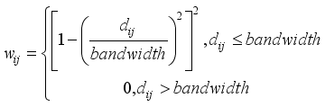 (1)
(1)  denotes the distance between County Unit
  and
and  , while
  represents the bandwidth parameter. Based on this weighting function, a local training set can be formed for each geographic unit
  by selecting its neighboring samples, upon which a localized random forest model is constructed
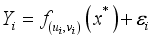
  can be expressed as
  , where represents the GW-RF prediction for I, and
  denotes the coordinates of center point
  :
:  (2)
(2) 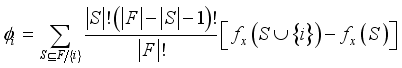 (3)
(3)  is a subset of features that does not include feature
  ,
,  denotes the model output when only the features in subset
  are used for prediction, and
  represents the total number of features.
  statistic and its corresponding
  -score for each county unit, one can determine whether a given region exhibits significant clustering of cultivated land fragmentation
  (4)
(4) 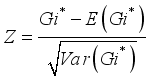 (5)
(5)  denotes the clustering index of county unit
  ;
;  represents the standardized value, reflecting the deviation between the expected value and the variance. When the
  -value is greater than 0 and the
  -value is less than 0.1, the location is identified as a hotspot; conversely, when the
  -value is less than 0 and the
  -value is less than 0.1, the location is identified as a cold spot.
 represents the
  extracted principal component, and its corresponding weight is the variance contribution rate of that component:
  (6)
(6) Indicator level | Indicator meaning |
|---|---|
PLAND | proportion of cropland area in the entire landscape (%) |
LPI | degree of cropland concentration (%) |
SHAPE_MN | shape complexity of cropland patches |
FRAC_MN | morphological complexity of cropland patches |
PARA_MN | irregularity of patches |
PLADJ | adjacency of same-type cropland |
COHESION | cropland connectivity (%) |
DIVISION | degree of landscape fragmentation |
AI | continuity of cropland distribution (%) |
 increased from 0.0139 in 1995 to a peak of 0.0208 in 2005, before gradually declining to 0.0112 by 2020. Although the overall trend of fragmentation at the national scale has moderated, localized fragmentation pressures have continued to intensify. During this period, the trajectories of cultivated land concentration, morphological complexity, and spatial connectivity diverged, resulting in a governance dilemma characterized by “macro-level improvement and micro-level deterioration.”
 Year | PLAND | LPI | SHAPE_MN | FRAC_MN | PARA_MN | PLADJ | COHESION | DIVISION | AI | LF |
|---|---|---|---|---|---|---|---|---|---|---|
1995 | 40.2 | 32.1 | 1.91 | 1.05 | 30.1 | 54.2 | 86.0 | 0.808 | 57.8 | 0.0139 |
2000 | 40.6 | 32.6 | 1.92 | 1.05 | 30.2 | 54.2 | 86.3 | 0.805 | 57.5 | 0.0194 |
2005 | 39.9 | 31.7 | 1.89 | 1.05 | 30.5 | 53.6 | 85.8 | 0.813 | 56.9 | 0.0208 |
2010 | 39.5 | 31.2 | 1.87 | 1.04 | 30.7 | 53.2 | 85.5 | 0.818 | 56.5 | 0.0205 |
2015 | 38.9 | 30.4 | 1.84 | 1.04 | 31.0 | 52.5 | 85.1 | 0.824 | 55.8 | 0.0196 |
2020 | 37.4 | 28.7 | 1.80 | 1.04 | 31.5 | 51.7 | 84.4 | 0.839 | 55.0 | 0.0112 |
1995 | 40.2 | 32.1 | 1.91 | 1.05 | 30.1 | 54.2 | 86.0 | 0.808 | 57.8 | 0.0139 |
Year | Moran’s I | P | Spatial autocorrelation diagnosis |
|---|---|---|---|
1995 | 0.8756 | 0.0000 | Significantly positive correlation |
2000 | 0.8736 | 0.0000 | Significantly positive correlation |
2005 | 0.8689 | 0.0000 | Significantly positive correlation |
2010 | 0.8650 | 0.0000 | Significantly positive correlation |
2015 | 0.8597 | 0.0000 | Significantly positive correlation |
2020 | 0.8527 | 0.0000 | Significantly positive correlation |
project | Precipitation | Temperature | Elevation | Slope | GDP | Population |
|---|---|---|---|---|---|---|
VIF1995 | 2.7267 | 3.3090 | 3.3956 | 2.7152 | 2.0951 | 2.1705 |
VIF2000 | 3.1507 | 3.5970 | 3.2616 | 2.8004 | 1.7909 | 1.8573 |
VIF2005 | 2.8242 | 3.0799 | 3.2943 | 2.7278 | 2.0352 | 1.9849 |
VIF2010 | 2.3174 | 2.4466 | 3.2502 | 2.7448 | 2.0890 | 1.9632 |
VIF2015 | 2.7539 | 3.2584 | 3.3385 | 2.6461 | 3.2871 | 3.3652 |
VIF2020 | 2.6272 | 2.9979 | 3.4849 | 2.6846 | 2.9722 | 3.0861 |
Variables/Indicators | %IncMSE | Minimum | Maximum | Mean | Standard |
|---|---|---|---|---|---|
Precipitation | 115.78 | 2.34 | 180.69 | 80.56 | 33.94 |
Temperature | 81.25 | 6.78 | 35.89 | 56.95 | 25.30 |
Elevation | 172.50 | -14.32 | 56.78 | 14.35 | 11.68 |
Slope | 180.65 | -3.85 | 55.06 | 21.94 | 10.22 |
GDP | 60.36 | 0.75 | 119.08 | 84.48 | 13.08 |
Population | 178.34 | 0.06 | 98.06 | 54.32 | 13.56 |
PLAND | Percentage of Landscape |
LPI | Largest Patch Index |
SHAPE_MN | Mean Shape Index |
FRAC_MN | Mean Patch Fractal Dimension |
PARA_MN | Mean Perimeter-Area Ratio |
PLADJ | Percentage of Like Adjacencies |
COHESION | Patch Cohesion Index |
DIVISION | Landscape Division Index |
AI | Aggregation Index |
YMLRR | Yangtze Middle and Lower Reaches Region |
YGPR | Yunan-Guizhou Plateau Region |
SBSA | Sichuan Basin and Surrounding Area |
QPTR | Qinghai-Tibet Plateau Region |
LP | Loess Plateau |
HHHPR | Huang-Huai-Hai Plain Region |
SCR | South China Region |
NCPR | Northern Arid and Semi arid Region |
LF | Landscape Fragmentation |
| [1] | Briones Alonso, E.; Cockx, L.; Swinnen, J. Culture and Food Security. Global Food Security 2018, 17, 113–127, |
| [2] | Xu, W.; Jin, X.; Liu, J.; Zhou, Y. Impact of Cultivated Land Fragmentation on Spatial Heterogeneity of Agricultural Agglomeration in China. J. Geogr. Sci. 2020, 30, 1571–1589, |
| [3] | Deng, F.; Jia, S.; Ye, M.; Li, Z. Coordinated Development of High-Quality Agricultural Transformation and Technological Innovation: A Case Study of Main Grain-Producing Areas, China. Environ Sci Pollut Res 2022, 29, 35150–35164, |
| [4] | Li, Y.; Wu, W.; Liu, Y. Land Consolidation for Rural Sustainability in China: Practical Reflections and Policy Implications. Land Use Policy 2018, 74, 137–141, |
| [5] | Zheng, B.; Gu, Y.; Zhu, H. Land Tenure Arrangements and Rural-to-Urban Migration: Evidence from Implementation of China’s Rural Land Contracting Law. Journal of Chinese Governance 2020, 5, 322–344, |
| [6] | Qu, L.; Liu, K.; Zhi, J.; Liu, W.; Fu, X.; Fan, T.; Wang, Z.; Zhou, Y. Spatiotemporal Dynamics and Driving Factors of Cultivated Land Fragmentation across China from 1990 to 2020. Landsc Ecol 2025. |
| [7] | Plexida, S. G.; Sfougaris, A. I.; Ispikoudis, I. P.; Papanastasis, V. P. Selecting Landscape Metrics as Indicators of Spatial Heterogeneity—A Comparison among Greek Landscapes. International Journal of Applied Earth Observation and Geoinformation 2014, 26, 26–35, |
| [8] | Long, J.; Nelson, T.; Wulder, M. Regionalization of Landscape Pattern Indices Using Multivariate Cluster Analysis. Environmental Management 2010, 46, 134–142, |
| [9] | Tan, S.; Heerink, N.; Kuyvenhoven, A.; Qu, F. Impact of Land Fragmentation on Rice Producers’ Technical Efficiency in South-East China. NJAS: Wageningen Journal of Life Sciences 2010, 57, 117–123, |
| [10] | Zeng, J.; Luo, T.; Gu, T.; Chen, W. How Does Cultivated Land Fragmentation Affect Soil Erosion: Evidence from the Yangtze River Basin in China. Journal of Environmental Management 2024, 360, 121020, |
| [11] | Zhou, Y.; Xu, K.; Feng, Z.; Wu, K. Quantification and Driving Mechanism of Cultivated Land Fragmentation under Scale Differences. Ecological Informatics 2023, 78, 102336, |
| [12] | Niroula, G. S.; Thapa, G. B. Impacts and Causes of Land Fragmentation, and Lessons Learned from Land Consolidation in South Asia. Land Use Policy 2005, 22, 358–372, |
| [13] | Manjunatha, A. V.; Anik, A. R.; Speelman, S.; Nuppenau, E. A. Impact of Land Fragmentation, Farm Size, Land Ownership and Crop Diversity on Profit and Efficiency of Irrigated Farms in India. Land Use Policy 2013, 31, 397–405, |
| [14] | Deininger, K.; Savastano, S.; Carletto, C. Land Fragmentation, Cropland Abandonment, and Land Market Operation in Albania. World Development 2012, 40, 2108–2122, |
| [15] | Liu, J.; Jin, X.; Xu, W.; Zhou, Y. Evolution of Cultivated Land Fragmentation and Its Driving Mechanism in Rural Development: A Case Study of Jiangsu Province. Journal of Rural Studies 2022, 91, 58–72, |
| [16] | Xu, W.; Jin, X.; Liu, J.; Zhou, Y. Analysis of Influencing Factors of Cultivated Land Fragmentation Based on Hierarchical Linear Model: A Case Study of Jiangsu Province, China. Land Use Policy 2021, 101, 105119, |
| [17] | Zhao, Y.; Feng, Q. Identifying Spatial and Temporal Dynamics and Driving Factors of Cultivated Land Fragmentation in Shaanxi Province. Agricultural Systems 2024, 217, 103948, |
| [18] | Ye, S.; Ren, S.; Song, C.; Du, Z.; Wang, K.; Du, B.; Cheng, F.; Zhu, D. Spatial Pattern of Cultivated Land Fragmentation in Mainland China: Characteristics, Dominant Factors, and Countermeasures. Land Use Policy 2024, 139, 107070, |
| [19] | Di Falco, S.; Penov, I.; Aleksiev, A.; Van Rensburg, T. M. Agrobiodiversity, Farm Profits and Land Fragmentation: Evidence from Bulgaria. Land Use Policy 2010, 27, 763–771, |
| [20] | Tan, S.; Heerink, N.; Qu, F. Land Fragmentation and Its Driving Forces in China. Land Use Policy 2006, 23, 272–285, |
| [21] | Hao, W.; Hu, X.; Wang, J.; Zhang, Z.; Shi, Z.; Zhou, H. The Impact of Farmland Fragmentation in China on Agricultural Productivity. Journal of Cleaner Production 2023, 425, 138962, |
| [22] | Ciaian, P.; Guri, F.; Rajcaniova, M.; Drabik, D.; Paloma, S. G. Y. Land Fragmentation and Production Diversification: A Case Study from Rural Albania. Land Use Policy 2018, 76, 589–599, |
| [23] | Qiu, L.; Zhu, J.; Pan, Y.; Wu, S.; Dang, Y.; Xu, B.; Yang, H. The Positive Impacts of Landscape Fragmentation on the Diversification of Agricultural Production in Zhejiang Province, China. Journal of Cleaner Production 2020, 251, 119722, |
| [24] | Quiñones, S.; Goyal, A.; Ahmed, Z. U. Geographically Weighted Machine Learning Model for Untangling Spatial Heterogeneity of Type 2 Diabetes Mellitus (T2D) Prevalence in the USA. Sci Rep 2021, 11, |
| [25] | Leong, Y.-Y.; Yue, J. C. A Modification to Geographically Weighted Regression. Int J Health Geogr 2017, 16, |
| [26] | Yu, Z.; Li, Z.; Yang, H.; Wang, Y.; Cui, Y.; Lei, G.; Ye, S. Contrasting Responses of Spatiotemporal Patterns of Cropland to Climate Change in Northeast China. Food Sec. 2023, 15, 1197–1214, |
| [27] | Antwarg, L.; Miller, R. M.; Shapira, B.; Rokach, L. Explaining Anomalies Detected by Autoencoders Using Shapley Additive Explanations. Expert Systems with Applications 2021, 186, 115736, |
| [28] | Chen, E.; Ye, Z.; Wu, H. Nonlinear Effects of Built Environment on Intermodal Transit Trips Considering Spatial Heterogeneity. Transportation Research Part D: Transport and Environment 2021, 90, 102677, |
| [29] | Liu, J.; Jin, X.; Xu, W.; Sun, R.; Han, B.; Yang, X.; Gu, Z.; Xu, C.; Sui, X.; Zhou, Y. Influential Factors and Classification of Cultivated Land Fragmentation, and Implications for Future Land Consolidation: A Case Study of Jiangsu Province in Eastern China. Land Use Policy 2019, 88, 104185, |
APA Style
Yaqing, W. (2025). Exploration of the Spatio-Temporal Evolution and Influencing Factors of Fragmentation of Cultivated Land in China. International Journal of Energy and Environmental Science, 10(5), 103-119. https://doi.org/10.11648/j.ijees.20251005.11
ACS Style
Yaqing, W. Exploration of the Spatio-Temporal Evolution and Influencing Factors of Fragmentation of Cultivated Land in China. Int. J. Energy Environ. Sci. 2025, 10(5), 103-119. doi: 10.11648/j.ijees.20251005.11
@article{10.11648/j.ijees.20251005.11,
  author = {Wu Yaqing},
  title = {Exploration of the Spatio-Temporal Evolution and Influencing Factors of Fragmentation of Cultivated Land in China
},
  journal = {International Journal of Energy and Environmental Science},
  volume = {10},
  number = {5},
  pages = {103-119},
  doi = {10.11648/j.ijees.20251005.11},
  url = {https://doi.org/10.11648/j.ijees.20251005.11},
  eprint = {https://article.sciencepublishinggroup.com/pdf/10.11648.j.ijees.20251005.11},
  abstract = {From the perspective of food security, cultivated land fragmentation is a major constraint to agricultural modernization. Based on 1-km resolution land use data from 1995 to 2020 in China, this study builds a comprehensive evaluation system and applies a Geographically Weighted Random Forest (GW-RF) model with SHAP interpretation to explore spatial-temporal patterns and the nonlinear, multi-factor drivers of fragmentation. Key findings include: (1) Fragmentation first intensified then eased, with clear regional differences—engineering efforts reduced fragmentation in the southwest by up to 18.7%, while urbanization and lagging land transfer increased it in the Huang-Huai-Hai region; the Qinghai-Tibet Plateau showed a unique “expansion–fluctuation” pattern under ecological policies. (2) Slope and population density are dominant nonlinear drivers, with threshold effects observed for precipitation, temperature, and elevation. For example, fragmentation rises sharply with slopes of 0–3° or population densities over 125 persons/km². (3) Spatial heterogeneity reveals that natural drivers vary by region and can be reshaped by policy—e.g., rainfall effects reversed in the southwest due to terracing, elevation constraints offset by farmland projects in Huang-Huai-Hai, and ecological policies reduced the impact of population density by 35% on the Plateau. The model highlights key thresholds (e.g., 800 mm rainfall, 3° slope) that support the need for region-specific governance.},
 year = {2025}
}
TY  - JOUR
T1  - Exploration of the Spatio-Temporal Evolution and Influencing Factors of Fragmentation of Cultivated Land in China

AU  - Wu Yaqing
Y1  - 2025/09/25
PY  - 2025
N1  - https://doi.org/10.11648/j.ijees.20251005.11
DO  - 10.11648/j.ijees.20251005.11
T2  - International Journal of Energy and Environmental Science
JF  - International Journal of Energy and Environmental Science
JO  - International Journal of Energy and Environmental Science
SP  - 103
EP  - 119
PB  - Science Publishing Group
SN  - 2578-9546
UR  - https://doi.org/10.11648/j.ijees.20251005.11
AB  - From the perspective of food security, cultivated land fragmentation is a major constraint to agricultural modernization. Based on 1-km resolution land use data from 1995 to 2020 in China, this study builds a comprehensive evaluation system and applies a Geographically Weighted Random Forest (GW-RF) model with SHAP interpretation to explore spatial-temporal patterns and the nonlinear, multi-factor drivers of fragmentation. Key findings include: (1) Fragmentation first intensified then eased, with clear regional differences—engineering efforts reduced fragmentation in the southwest by up to 18.7%, while urbanization and lagging land transfer increased it in the Huang-Huai-Hai region; the Qinghai-Tibet Plateau showed a unique “expansion–fluctuation” pattern under ecological policies. (2) Slope and population density are dominant nonlinear drivers, with threshold effects observed for precipitation, temperature, and elevation. For example, fragmentation rises sharply with slopes of 0–3° or population densities over 125 persons/km². (3) Spatial heterogeneity reveals that natural drivers vary by region and can be reshaped by policy—e.g., rainfall effects reversed in the southwest due to terracing, elevation constraints offset by farmland projects in Huang-Huai-Hai, and ecological policies reduced the impact of population density by 35% on the Plateau. The model highlights key thresholds (e.g., 800 mm rainfall, 3° slope) that support the need for region-specific governance.
VL  - 10
IS  - 5
ER  -
School of Mathematics and Statistics, Hunan University of Technology and Business, Changsha, China
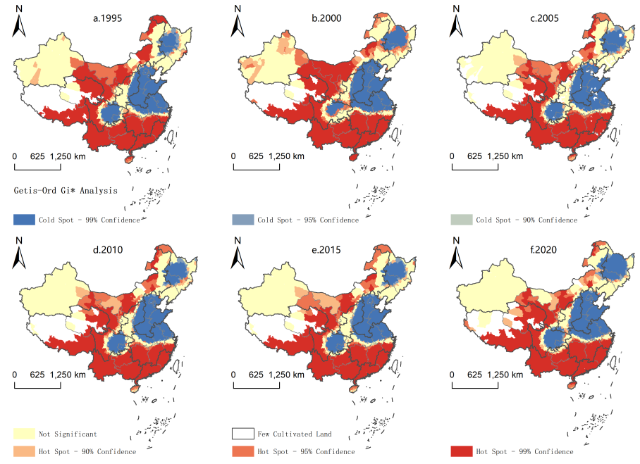
Figure 1. Spatiotemporal Evolution of Farmland Fragmentation in Major Agricultural Regions of China.
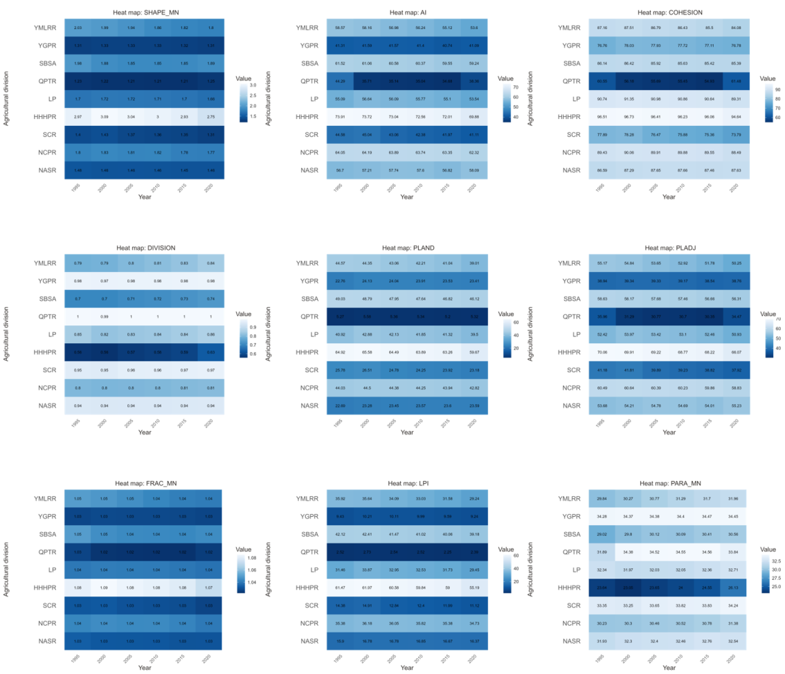
Figure 2. Landscape fragmentation in nine major agricultural areas of China from 1995 to 2020.
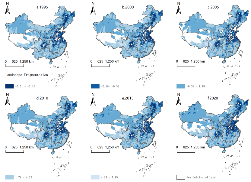
Figure 3. The rate of landscape fragmentation at county level in China from 1995 to 2020.
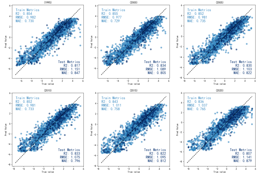
Figure 4. The fitted scatter plot of the GW-RF model.
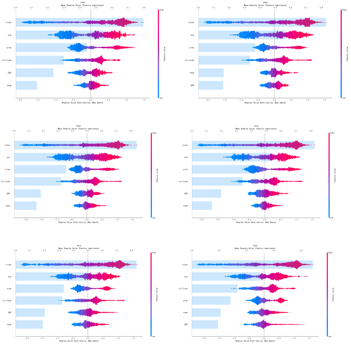
Figure 5. Global interpretation graph.
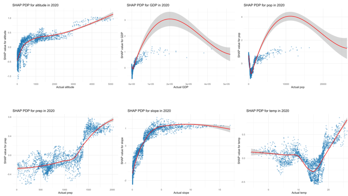
Figure 6. SHAP-PDP graph.
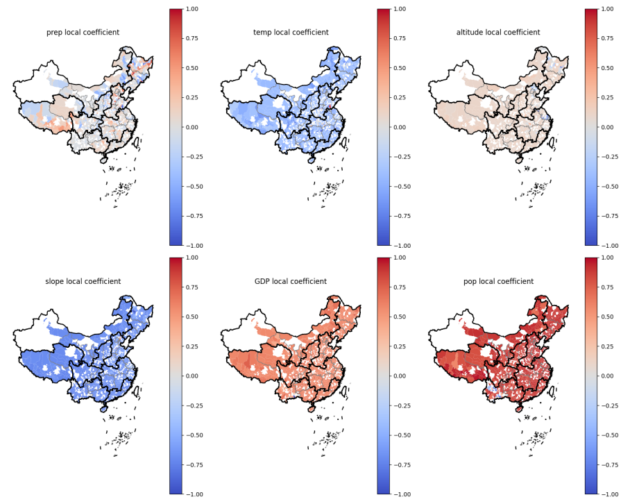
Figure 7. Local coefficient diagram of GW-RF model.
Information